
Introduction to Polynomials
What Are Polynomials?
A polynomial is an expression containing constants and variables connected only through basic operations of algebra.Learning Objectives
Describe what polynomials are and their defining characteristicsKey Takeaways
Key Points
- A polynomial is a finite expression constructed from variables and constants, using the operations of addition, subtraction, multiplication, and taking non-negative integer powers.
- A polynomial can be written as the sum of a finite number of terms. Each term consists of the product of a constant (called the coefficient of the term) and a finite number of variables (usually represented by letters) raised to integer powers.
Key Terms
- polynomial: an expression consisting of a sum of a finite number of terms, each term being the product of a constant coefficient and one or more variables raised to a non-negative integer power, such as [latex]a_n x^n + a_{n-1}x^{n-1} +... + a_0 x^0[/latex].
- degree: the sum of the exponents of a term; the order of a polynomial.
- coefficient: a constant by which an algebraic term is multiplied.
Monomials over [latex]\mathbb{R}[/latex]
Let [latex]\mathbb{R}[/latex] be the set of real numbers. A monomial over [latex]\mathbb{R}[/latex] in a single variable [latex]x[/latex] consists of a non-negative power of [latex]x[/latex], multiplied with a nonzero constant [latex]c \in \mathbb{R}.[/latex] So a polynomial looks like [latex]cx^n[/latex], where [latex]n \geq 0[/latex] is an integer and [latex]c \not = 0[/latex] is a real number. If we want to give the polynomial a name, say [latex]M[/latex], we denote that its variable is [latex]x[/latex] by writing [latex]x[/latex] between brackets: [latex]M(x)=cx^n[/latex]. The exponent [latex]n[/latex] is called the degree of [latex]M(x).[/latex] The constant [latex]c[/latex] is the coefficient.Examples
[latex]\sqrt{2}x^7[/latex]is a monomial of degree 7 and coefficient [latex]\sqrt{2}[/latex]. [latex]7x^{\sqrt{2}}[/latex], [latex]\sqrt{2}x^{-7}[/latex] and [latex]2x^7 - 7x^2[/latex]are not monomials. The first and the second do not have a non-negative integer exponent and the third is a sum of two monomials.Polynomials over [latex]\mathbb{R}[/latex]
A polynomial over [latex]\mathbb{R}[/latex] is a finite sum of monomials over [latex]\mathbb{R}[/latex]. For example [latex-display]P(x)= 4x^{13} +3x^2-\pi x + 1[/latex-display] is the finite sum of the [latex]4[/latex] monomials: [latex]4x^{13}, 3x^2, -\pi x[/latex] and [latex]1 = 1x^0.[/latex] It is also the sum of the 6 monomials: [latex]1/3 x^{100}, -1/3 x^{100}, 4x^{13}, 3x^2, -\pi x[/latex] and [latex]1[/latex], as will be explained in the discussion about addition and subtraction of polynomials. However, we can only write down [latex]P(x)[/latex] as the sum of monomials of distinct degree in exactly one way, namely the first we mentioned. These monomials are called the terms of [latex]P(x).[/latex]The coefficients of [latex]P(x)[/latex] are the coefficients corresponding to its terms. Every monomial is also a polynomial, as it can be written as a sum with one term, itself. A special example of a polynomial is the zero polynomial [latex-display]Z(x) = 0,[/latex-display] which is a sum of [latex]0[/latex] monomials. The degree of a polynomial [latex]Q(x)[/latex] is the highest degree of one of its terms. For example, the degree of [latex]P(x)[/latex] is [latex]13[/latex]. The degree of the zero polynomial is defined to be [latex]-\infty[/latex].Extra: Polynomials Over General Rings
This part is for the interested reader only. Most students can skip this part, or just remember that polynomials over [latex]\mathbb{C}[/latex] are the same as polynomials over [latex]\mathbb{R}[/latex], but with complex coefficients and that the degree of a monomial in more variables equals the sum of the exponents. We have discussed polynomials over [latex]\mathbb{R}[/latex]. We shall later see that we can add, subtract and multiply these polynomials. In general, our coefficients [latex]c[/latex] do not need to belong to [latex]\mathbb{R}[/latex], but they can belong to any set of "numbers" in which we can add, subtract and multiply. These sets are called rings. Examples of rings are the real numbers [latex]\mathbb{R}[/latex], the integers [latex]\mathbb{Z}[/latex] and the complex numbers [latex]\mathbb{C}[/latex]. In this case, we talk about complex polynomials, or polynomials over [latex]\mathbb{C}[/latex]. The degree of a polynomial is defined in the same way as in the real case. In particular, the polynomials over [latex]\mathbb{R}[/latex] form a ring, which we denote by [latex]\mathbb{R}[x][/latex]. The polynomials over this ring will be polynomials in two variables [latex]x[/latex] and [latex]y[/latex] over [latex]\mathbb{R}[/latex]. Here the degree in [latex]x[/latex] of [latex]x^3y^5[/latex]is [latex]3[/latex], the degree in [latex]y[/latex] of [latex]x^3y^5[/latex]is [latex]5[/latex] and its joint degree or degree is [latex]8[/latex].Adding and Subtracting Polynomials
Polynomials can be added or subtracted by combining like terms.Learning Objectives
Explain how to add and subtract polynomials and what it means to do soKey Takeaways
Key Points
- The rules for adding and subtracting algebraic expressions apply to polynomials; only like terms can be combined.
- Any two polynomials can be added or subtracted, regardless of the number of terms in each, or the degrees of the polynomials.
- The sum or difference of two polynomials will have the same degree as the polynomial with the higher degree in the problem.
Key Terms
- Commutative Property: States that changing the order of numbers being added does not change the result.
- degree of a polynomial: The highest value of an exponent placed on a variable in any of the terms of a polynomial.
Example 1
Find the sum of [latex]4x^2 - 5x + 1[/latex] and [latex]3x^2 - 8x - 9[/latex]. First, group like terms together: [latex-display](4x^2 +3x^2 ) + (- 5x-8x) + (1 - 9)[/latex-display] Combine the like terms for the solution: [latex-display]7x^2 - 13x - 8[/latex-display]Example 2
Subtract: [latex](5x^3 + x^2 + 9) - (4x^2 + 7x -3)[/latex] Start by grouping like terms. Remember to apply subtraction to each term in the second polynomial. Note that the term [latex]5x^3[/latex] in the first polynomial does not have a like term; neither does [latex]7x[/latex] in the second polynomial. These are simply carried down. [latex]5x^3 + (x^2 - 4x^2) + (- 7x) + (9 - (-3)) \\ 5x^3 + (x^2 - 4x^2) - 7x +(9 + 3)[/latex] Now combine the like terms: [latex-display]5x^3 - 3x^2 - 7x + 12[/latex-display] Notice that the answer is a polynomial of degree 3; this is also the highest degree of a polynomial in the problem.Multiplying Polynomials
To multiply two polynomials together, multiply every term of one polynomial by every term of the other polynomial.Learning Objectives
Explain how to multiply polynomials using the distributive property and describe the results of doing soKey Takeaways
Key Points
- To multiply a polynomial by a monomial, multiply every term of the polynomial by the monomial and then add the resulting products together.
- To multiply two polynomials together, multiply every term of one polynomial by every term of the other polynomial.
- The degree of a product of two polynomials equals the sum of the degrees of said polynomials.
- The zeros of a product of two polynomial are the zeros of the two factors, combined.
Key Terms
- monomial: An algebraic expression consisting of one term.
- commutative: A binary operation is commutative if changing the order of the operands does not change the result, for example addition and multiplication.
- polynomial: an expression consisting of a sum of a finite number of terms, each term being the product of a constant coefficient and one or more variables raised to a non-negative integer power, such as [latex]a_n x^n + a_{n-1}x^{n-1} +... + a_0 x^0[/latex]. Importantly, because all exponents are positive, it is impossible to divide by [latex]x[/latex].
Zeros of a Product of Polynomials
Since we made sure that the product of polynomials abides the same laws as if the variables were real numbers, the evaluation of a product of two polynomials in a given point will be the same as the product of the evaluations of the polynomials: [latex-display]P(x_0)Q(x_0) = PQ(x_0)[/latex-display] for all real numbers [latex]x_0.[/latex] In particular [latex]PQ(x_0) = 0[/latex] if and only if [latex]P(x_0)Q(x_0)=0[/latex], if and only if [latex]P(x_0) = 0[/latex] or [latex]Q(x_0) = 0[/latex]. So the roots of a product of polynomials are exactly the roots of its factors, i.e. [latex]x_0[/latex] is a zero for [latex]PQ(x)[/latex] if it is a zero for [latex]P(x)[/latex] or for [latex]Q(x)[/latex] (and possibly both).Polynomial and Rational Functions as Models
Functions are commonly used in fitting data to a trend line. Polynomial and rational functions are both relatively accurate and easy to use.Learning Objectives
Discuss the advantages and disadvantages of using polynomial and rational functions as modelsKey Takeaways
Key Points
- Researchers will often collect many discrete samples of data, relating two or more variables, without knowing the mathematical relationship between them. Curve fitting is used to create trend lines intended to fill in the points between and beyond collected data points.
- Polynomial functions are easy to use for modeling, but ill-suited to modeling asymptotes and some functional forms, and they can become very inaccurate outside the bounds of the collected data.
- Rational functions can take on a much greater range of shapes and are more accurate both inside and outside the limits of collected data than polynomial functions. However, rational functions are more difficult to use and can include undesirable asymptotes.
Key Terms
- asymptote: A line that a curve approaches arbitrarily closely, as they go to infinity; the limit of the curve, its tangent "at infinity".
- They are well studied: a lot of their properties are known.
- They are easy to compute, using only multiplication and addition.
- They are closed under rescaling or changing of locations: if we change a kilometer to a mile we still get a polynomial.
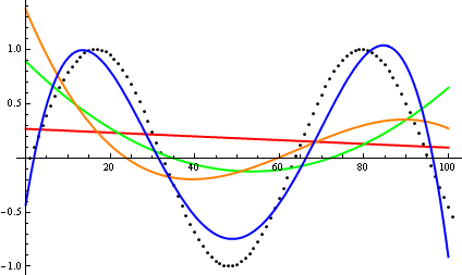 Curve fitting: Polynomial curves generated to fit points (black dots) of a sine function: The red line is a first degree polynomial; the green is a second degree; the orange is a third degree; and the blue is a fourth degree.
Polynomials and rational functions are used for approximation in many everyday devices. For example, every time we take a picture with a smartphone, our phone looks at some data points and fills in the appropriate colors in the blanks, thus saving us a lot of memory, with the help of rational functions. Every time we say something through the phone, our phone tries to reduce the background noise by approximating our sound for short periods of time, again with the help of rational functions.
Licenses & Attributions
CC licensed content, Shared previously
- Curation and Revision. Authored by: Boundless.com. License: Public Domain: No Known Copyright.
CC licensed content, Specific attribution
- Polynomial. Provided by: Wikipedia License: CC BY-SA: Attribution-ShareAlike.
- degree. Provided by: Wiktionary License: CC BY-SA: Attribution-ShareAlike.
- polynomial. Provided by: Wiktionary License: CC BY-SA: Attribution-ShareAlike.
- coefficient. Provided by: Wiktionary License: CC BY-SA: Attribution-ShareAlike.
- Adding and Subtracting Algebraic Expressions. Provided by: Boundless License: CC BY-SA: Attribution-ShareAlike.
- Commutative property. Provided by: Wikipedia License: CC BY-SA: Attribution-ShareAlike.
- Add and Subtract Polynomials. Provided by: OpenStax Located at: https://cnx.org/contents/31d9fc9e-aa3b-4506-ad7a-5559ba9e8c87@6. License: CC BY: Attribution.
- Oka Kurniawan, Basic Mathematics Review. September 17, 2013. Provided by: OpenStax CNX License: CC BY: Attribution.
- Wade Ellis and Denny Burzynski, Elementary Algebra. September 17, 2013. Provided by: OpenStax CNX Located at: https://cnx.org/contents/[email protected]:d083791f-1d4a-4a36-b069-9aff3b1bbf74. License: CC BY: Attribution.
- polynomial. Provided by: Wiktionary License: CC BY-SA: Attribution-ShareAlike.
- monomial. Provided by: Wiktionary License: CC BY-SA: Attribution-ShareAlike.
- commutative. Provided by: Wiktionary License: CC BY-SA: Attribution-ShareAlike.
- Rational functions. Provided by: wikipedia License: CC BY-SA: Attribution-ShareAlike.
- Polynomial and rational function modeling. Provided by: Wikipedia Located at: https://en.wikipedia.org/wiki/Polynomial_and_rational_function_modeling. License: CC BY-SA: Attribution-ShareAlike.
- asymptote. Provided by: Wiktionary License: CC BY-SA: Attribution-ShareAlike.
- Curve fitting. Provided by: Wikipedia License: CC BY-SA: Attribution-ShareAlike.
