
Zeroes of Polynomial Functions
The Fundamental Theorem of Algebra
The fundamental theorem states that every non-constant, single-variable polynomial with complex coefficients has at least one complex root.Learning Objectives
Discuss the fundamental theorem of algebraKey Takeaways
Key Points
- The fundamental theorem of algebra states that every non-constant, single- variable polynomial with complex coefficients has at least one complex root. This includes polynomials with real coefficients, since every real number is a complex number with zero as its coefficient.
- The fundamental theorem is also stated as follows: every non-zero, single-variable, degree [latex]n[/latex] polynomial with complex coefficients has, counted with multiplicity, exactly [latex]n[/latex] roots. The equivalence of the two statements can be proven through the use of successive polynomial division.
Key Terms
- multiplicity: the number of values for which a given condition holds
The Fundamental Theorem
The fundamental theorem of algebra says that every non-constant polynomial in a single variable [latex]z[/latex], so any polynomial of the form [latex-display]c_nx^n + c_{n-1}x^{n-1} + \ldots c_0[/latex-display] where [latex]n > 0[/latex] and [latex]c_n \not = 0[/latex], has at least one complex root. There are lots of proofs of the fundamental theorem of algebra. However, despite its name, no purely algebraic proof exists, since every proof makes use of the fact that [latex]\mathbb{C}[/latex] is complete. In particular, since every real number is also a complex number, every polynomial with real coefficients does admit a complex root. For example, the polynomial [latex]x^2 + 1[/latex] has [latex]i[/latex] as a root.Alternative Statement
Saying that [latex]x_0[/latex] is a root of a polynomial [latex]f(x)[/latex] is the same as saying that [latex](x-x_0)[/latex] divides [latex]f(x).[/latex] We say that a root [latex]x_0[/latex] has multiplicity [latex]m[/latex] if [latex](x-x_0)^m[/latex] divides [latex]f(x)[/latex] but [latex](x-x_0)^{m+1}[/latex] does not. For example, the polynomial [latex-display]x^4(x-i)^3(x+\pi)[/latex-display] admits one complex root of multiplicity [latex]4[/latex], namely [latex]x_0 = 0[/latex], one complex root of multiplicity [latex]3[/latex], namely [latex]x_1 = i[/latex], and one complex root of multiplicity [latex]1[/latex], namely [latex]x_2 = - \pi[/latex]. The sum of the multiplicity of the roots equals the degree of the polynomial, [latex]8[/latex]. For non-zero complex polynomials, this turns out to be true in general and follows directly from the fundamental theorem of algebra. Indeed, a polynomial of degree [latex]0[/latex] takes on the form [latex]c_0[/latex], where [latex]c_0 \not = 0[/latex], and thus has no zeros. For a general polynomial [latex]f(x)[/latex] of degree [latex]n[/latex], the fundamental theorem of algebra says that we can find one root [latex]x_0[/latex] of [latex]f(x)[/latex]. Thus we can factor [latex]f(x)[/latex] as [latex-display]f(x) = (x-x_0)f_1(x)[/latex-display] where [latex]f_1(x)[/latex] is a non-zero polynomial of degree [latex]n-1.[/latex] So if the multiplicities of the roots of [latex]f_1(x)[/latex] add to [latex]n-1[/latex], the multiplicity of the roots of [latex]f[/latex] add to [latex]n[/latex]. So since the property is true for all polynomials of degree [latex]0[/latex], it is also true for all polynomials of degree [latex]1[/latex]. And since it is true for all polynomials of degree [latex]1[/latex], it is also true for all polynomials of degree [latex]2[/latex]. In general, for any [latex]n \in \mathbb{N}[/latex], we will be able to conclude that the property is true for all polynomials of degree [latex]n.[/latex] Thus the property is true for all polynomials. Conversely, if the multiplicities of the roots of a polynomial add to its degree, and if its degree is at least [latex]1[/latex] (i.e. it is not constant), then it follows that it has at least one zero. So an alternative statement of the fundamental theorem of algebra is: The multiplicities of the complex roots of a nonzero polynomial with complex coefficients add to the degree of said polynomial.The Complex Conjugate Root Theorem
The complex conjugate root theorem says that if a complex number [latex]a+bi[/latex] is a zero of a polynomial with real coefficients, then its complex conjugate [latex]a-bi[/latex] is also a zero of this polynomial. Now suppose our real polynomial admits a root [latex]a+bi[/latex] with [latex]b \not = 0[/latex]. By dividing with the real polynomial[latex](x-(a+bi))(x-(a-bi))=(x-a)^2 +b^2[/latex], we obtain another real polynomial, for which the complex conjugate root theorem again applies. In this way, we see that the total multiplicity of non-real complex roots of a polynomial with real coefficients must always be even. This last remark, together with the alternative statement of the fundamental theorem of algebra, tells us that the parity of the real roots (counted with multiplicity) of a polynomial with real coefficients must be the same as the parity of the degree of said polynomial. Therefore, a polynomial of even degree admits an even number of real roots, and a polynomial of odd degree admits an odd number of real roots (counted with multiplicity). In particular, every polynomial of odd degree with real coefficients admits at least one real root.[latex][/latex]Finding Polynomials with Given Zeros
To construct a polynomial from given zeros, set [latex]x[/latex] equal to each zero, move everything to one side, then multiply each resulting equation.Learning Objectives
Use the zeros of a polynomial to write a polynomial with those zerosKey Takeaways
Key Points
- A polynomial constructed from [latex]n[/latex] roots will have degree [latex]n[/latex] or less. That is to say, if given three roots, then the highest exponential term needed will be [latex]x^3[/latex].
- Each zero given will end up being one term of the factored polynomial. After finding all the factored terms, simply multiply them together to obtain the whole polynomial.
- Because a polynomial and a polynomial multiplied by a constant have the same roots, every time a polynomial is constructed from given zeros, the general solution includes a constant, shown here as [latex]c[/latex].
Key Terms
- polynomial: An expression consisting of a sum of a finite number of terms, each term being the product of a constant coefficient and one or more variables raised to a non-negative integer power, such as [latex]a_n x^n + a_{n-1}x^{n-1} +... + a_0 x^0[/latex]. Importantly, because all exponents are positive, it is impossible to divide by [latex]x[/latex].
- zero: Also known as a root, a zero is an [latex]x[/latex] value at which the function of [latex]x[/latex] is equal to [latex]0[/latex].
Degree of the Polynomial
Remember that the degree of a polynomial, the highest exponent, dictates the maximum number of roots it can have. Thus, the degree of a polynomial with a given number of roots is equal to or greater than the number of roots that are given. If we already count multiplicity in this number, than the degree equals the number of roots. For example, if we are given two zeros, then a polynomial of second degree needs to be constructed.Solution and Constants
If [latex]x_1, x_2, \ldots x_n[/latex] are the zeros of [latex]f(x)[/latex] and the leading coefficient of [latex]f(x)[/latex] is [latex]1[/latex], then [latex]f(x)[/latex] factorizes as [latex-display]f(x)=(x-x_1)(x-x_2)\cdots(x-x_n)[/latex-display] This already gives us the solution of our problem: an answer to our question is just the product of all factors [latex](x-x_i)[/latex], where the [latex]x_i[/latex] are the given zeros! However, we see that this polynomial is not unique: For any nonzero constant [latex]a[/latex], we have that [latex](af)(x)=af(x)[/latex] factorizes as [latex-display]af(x) = a(x-x_1)(x-x_2) \cdots (x-x_n)[/latex-display] Thus if we find a solution [latex]g(x)[/latex] for our problem, we have actually found infinitely many solutions [latex]cg(x)[/latex], one for every non-zero number [latex]c[/latex]. Thus for given zeros [latex]x_1, x_2, \ldots, x_n[/latex] we find infinitely many solutions [latex-display]c(x-x_1)(x-x_2)\cdots (x-x_n)[/latex-display] For example, if given [latex]a[/latex] and [latex]b[/latex] as zeros, then the resulting initial terms would be a constant [latex]c[/latex] times the two factors that give zeros at the appropriate place: [latex-display]c(x-a)(x-b)[/latex-display] Multiplied out, this gives: [latex-display]cx^2-c(a+b)x+abc[/latex-display]Example
Given zeros [latex]0[/latex], [latex]1[/latex], and [latex]2[/latex], our general solution is of the form [latex-display]cx(x-1)(x-2) = cx^3 - 3cx^2 + 2cx[/latex-display] In the picture below, the blue graph represents the solution for [latex]c[/latex] equal to [latex]1[/latex]. The red graph represents the solution for [latex]c[/latex] equal to [latex]-1/2[/latex].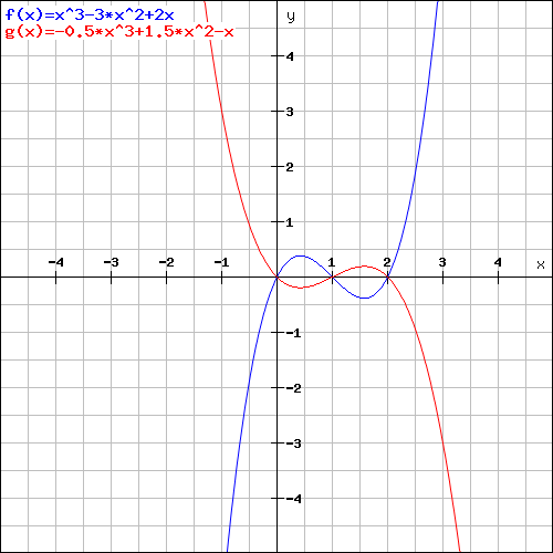 Example: Two polynomials with the same zeros: Both [latex]f(x)[/latex] and [latex]g(x)[/latex] have zeros [latex]0, 1[/latex] and [latex]2[/latex]. They are equal up to a constant. Changing the value and sign of the constant does not change the zeroes, since zero multiplied by any constant is still zero.
Finding Zeros of Factored Polynomials
The factored form of a polynomial reveals its zeros, which are defined as points where the function touches the [latex]x[/latex]-axis.Learning Objectives
Use the factored form of a polynomial to find its zerosKey Takeaways
Key Points
- A polynomial function may have zero, one, or many zeros.
- All polynomial functions of positive, odd order have at least one zero, while polynomial functions of positive, even order may not have a zero.
- Regardless of odd or even, any polynomial of positive order can have a maximum number of zeros equal to its order.
Key Terms
- zero: Also known as a root, a zero is an [latex]x[/latex] value at which the function of [latex]x[/latex] is equal to [latex]0[/latex].
Number of Zeros of a Polynomial
Consider the factored function: [latex-display]f(x)=(x-a_1)(x-a_2)...(x-a_n)[/latex-display] Each value [latex]a_1,a_2[/latex], and so on is a zero. A polynomial function may have many, one, or no zeros. All polynomial functions of positive, odd order have at least one zero (this follows from the fundamental theorem of algebra), while polynomial functions of positive, even order may not have a zero (for example [latex]x^4+1[/latex] has no real zero, although it does have complex ones). Regardless of odd or even, any polynomial of positive order can have a maximum number of zeros equal to its order. For example, a cubic function can have as many as three zeros, but no more. This is known as the fundamental theorem of algebra.Example
Consider the function [latex-display]f(x)=x^3+2x^2-5x-6[/latex-display] This can be rewritten in factored form: [latex-display]f(x)=(x+3)(x+1)(x-2)[/latex-display] Replacing [latex]x[/latex] with a value that will make either [latex](x+3),(x+1)[/latex] or [latex](x-2)[/latex] zero will result in [latex]f(x)[/latex] being equal to zero. Thus, the zeros for [latex]f(x)[/latex] are at [latex]x=-3,x=-1[/latex] and [latex]x=2.[/latex] This can also be shown graphically: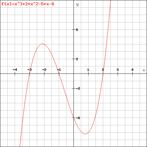 Cubic function: Graph of the cubic function [latex]f(x) = x^3 + 2x^2 - 5x - 6 = (x+3)(x+1)(x-2).[/latex] We see that its roots equal the negative second coefficients of its first degree factors
Factoring and zeros
In general, we know from the remainder theorem that [latex]a[/latex] is a zero of [latex]f(x)[/latex] if and only if [latex]x-a[/latex] divides [latex]f(x).[/latex] Thus if we can factor [latex]f(x)[/latex] in polynomials of as small a degree as possible, we know its zeros by looking at all linear terms in the factorization. This is why factorization is so important: to be able to recognize the zeros of a polynomial quickly. It follows from the fundamental theorem of algebra and a fact called the complex conjugate root theorem, that every polynomial with real coefficients can be factorized into linear polynomials and quadratic polynomials without real roots. Thus if you have found such a factorization of a given function, you can be completely sure what the zeros of that function are.Integer Coefficients and the Rational Zeros Theorem
Each solution to a polynomial, expressed as [latex]x= \frac {p}{q}[/latex], must satisfy that [latex]p[/latex] and [latex]q[/latex] are integer factors of [latex]a_0[/latex] and [latex]a_n[/latex], respectively.Learning Objectives
Use the Rational Zeros Theorem to find all possible rational roots of a polynomialKey Takeaways
Key Points
- In algebra, the Rational Zeros Theorem (also known as the Rational Root Theorem, or the Rational Root Test) states a constraint on rational solutions (or roots) of the polynomial equation [latex]a_nx^n+a_{n-1}x^{n-1}+...+a_0=0[/latex] with integer coefficients.
- If [latex]a_0[/latex] and [latex]a_n[/latex] are non-zero, then each rational solution [latex]x[/latex], when written as a fraction [latex]x= \frac {p}{q}[/latex] in lowest terms (i.e., the greatest common divisor of [latex]p[/latex] and [latex]q[/latex] is [latex]1[/latex]), satisfies the following: [latex]1[/latex]) [latex]p[/latex] is an integer factor of the constant term [latex]a_0[/latex], and [latex]2[/latex]) [latex]q[/latex] is an integer factor of the leading coefficient [latex]a_n[/latex].
Key Terms
- Euclid's lemma: One of the fundamental properties of prime numbers. States that if a prime divides the product of two numbers, it must divide at least one of the factors. For example since 133 × 143 = 19019 is divisible by 19, one or both of 133 or 143 must be as well. In fact, 19 × 7 = 133. It is used in the proof of the fundamental theorem of arithmetic.
- coprime: Having no positive integer factors, aside from [latex]1[/latex], in common with one or more specified other positive integers.
The Rational Zero Theorem
In algebra, the Rational Zero Theorem, or Rational Root Theorem, or Rational Root Test, states a constraint on rational solutions (also known as zeros, or roots) of the polynomial equation [latex-display]a_nx^n+a_{n-1}x^{n-1}+...+a_0=0[/latex-display] With integer coefficients [latex]a_n,a_{n-1},\ldots,a_0.[/latex] If [latex]a_0[/latex] and [latex]a_n[/latex] are nonzero, then each rational solution [latex]x= \frac {p}{q}[/latex], where [latex]p[/latex] and [latex]q[/latex] are coprime integers (i.e. their greatest common divisor is [latex]1[/latex]), satisfies:- [latex]p[/latex] is a divisor of the constant term [latex]a_0[/latex].
- [latex]q[/latex] is a divisor of the leading coefficient [latex]a_n[/latex].
Example
For example, every rational solution of the cubic equation [latex-display]3x^3-5x^2+5x-2=0[/latex-display] must be among the numbers symbolically indicated by: [latex-display]\pm \frac {1,2}{1,3}[/latex-display]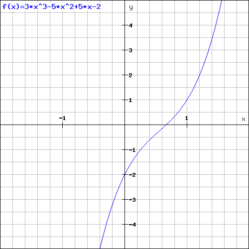 Cubic function: The cubic function [latex]3x^3-5x^2+5x-2[/latex] has one real root between [latex]0[/latex] and [latex]1[/latex]. We can use the Rational Root Test to see whether this root is rational.
i.e. its numerator must divide [latex]2[/latex] and its denominator must divide [latex]3[/latex]. This gives the list of possible answers
[latex-display]1,-1,2,-2,\frac 13, -\frac 13, \frac 23, -\frac 23[/latex-display] These root candidates can be tested, either by plugging them in directly, or by dividing and checking to see whether there is any remainder, for example using long division. The advantage of this is that once we have found a root, we immediately have found the smaller degree polynomial of which we again wish to find the roots and the rational root theorem will provide us with even fewer candidates for this root. Moreover, once we have established a root, we must use division anyway to check whether it is a multiple root. The disadvantage is that we have to use long division more often. When there are a lot of zero candidates for a small degree polynomial, we may just want to plug in candidates and only use division when we have found a root. In our example, we can plug in [latex]x_0=1[/latex] to see that it is not a root. In fact, the left hand value is equal to [latex]1[/latex]. Now we use a little trick: since the constant term of [latex](x-x_0)^k[/latex] equals [latex]x_0^k[/latex] for all positive integers [latex]k[/latex], we can substitute [latex]x[/latex] by [latex]t+x_0[/latex] to find a polynomial with the same leading coefficient as our original polynomial and a constant term equal to the value of the polynomial at [latex]x_0[/latex]. In this case we substitute [latex]x[/latex] with [latex]t+1[/latex] and obtain a polynomial in [latex]t[/latex] with leading coefficient [latex]3[/latex] and constant term [latex]1[/latex]. Thus the candidates for zeros in this polynomial in [latex]t[/latex] are [latex-display]t=\pm \frac 1{1,3}[/latex-display] Thus the candidates for roots of the polynomial in [latex]x[/latex] must be one greater than one of these candidates: [latex-display]x=1+t=2,0,\frac 43, \frac 23[/latex-display] Root candidates that do not occur on both lists are ruled out. The list of rational root candidates has thus shrunk to just [latex]x=2[/latex] and [latex]x=2/3[/latex]. After checking for these candidates, we see that the only rational root (with multiplicity [latex]1)[/latex] is [latex]2/3[/latex], which can also be seen in the graph above.The Rule of Signs
The rule of signs gives an upper bound number of positive or negative roots of a polynomial.Learning Objectives
Use the rule of signs to find out the maximum number of positive and negative roots a polynomial hasKey Takeaways
Key Points
- The rule of signs gives us an upper bound number of positive or negative roots of a polynomial. It is not a complete criterion, meaning that it does not tell the exact number of positive or negative roots.
- The rule states that if the terms of a polynomial with real coefficients are ordered by descending variable exponent, then the number of positive roots of the polynomial is either equal to the number of sign differences between consecutive nonzero coefficients, or is less by a multiple of 2.
- As a corollary of the rule, the number of negative roots is the number of sign changes after multiplying the coefficients of odd-power terms by [latex]-1[/latex], or less by a multiple of 2.
Key Terms
- sign: positive or negative polarity.
- root: any number which, when plugged into the equation, will produce a zero.
Positive Roots
In order to find the number of positive roots in a polynomial with only one variable, we must first arrange the polynomial by descending variable exponent. For example, [latex]-x^2 + x^3 + x[/latex] would be written [latex]x^3 - x^2 + x[/latex]. Then, we must count the number of sign differences between consecutive nonzero coefficients. This number, or any number less than it by a multiple of 2, could be the number of positive roots. In the example [latex]x^3 - x^2 + x[/latex], there are two sign changes, after the first and second terms. Thus, there are either two or zero positive roots for this polynomial. It is important to note that for polynomials with multiple roots of the same value, each of these roots is counted separately.Negative Roots
Finding the negative roots is similar to finding the positive roots. The difference is that you must start by finding the coefficients of odd power (for example, [latex]x^3[/latex] or [latex]x^5[/latex], but not [latex]x^2[/latex] or [latex]x^4[/latex]). Once you have located them, multiply each by [latex]-1[/latex]. Then the procedure is the same; count the number of sign changes between consecutive nonzero coefficients. This number, or any number less than it by a multiple of 2, could be your number of negative roots. Again it is important to note that multiple roots of the same value should be counted separately. This can also be done by taking the function, [latex]f(x)[/latex], and substituting the [latex]x[/latex] for [latex]-x[/latex], so that we have the function [latex]f(-x)[/latex]. The reason we only bother to change the sign of the odd power coefficients is because if we substitute in [latex]-x[/latex] in an even power, it will just become a positive again. For example: [latex](-x)^3 = (-x)(-x)(-x) = -x^3[/latex] but [latex](-x)^2 = (-x)(-x) = x^2[/latex] We can see that the negative signs cancel out for any even power. By only multiplying the odd powered coefficients by [latex]-1[/latex], we are essentially saving ourselves a step.Example
Consider the polynomial: [latex-display]f(x)=x^3+x^2-x-1[/latex-display] This function has one sign change between the second and third terms. Therefore it has exactly one positive root. Don't forget that the first term has a sign, which, in this case, is positive. Next, we move on to finding the negative roots. Change the exponents of the odd-powered coefficients, remembering to change the sign of the first term. Once you have done this, you have obtained the second polynomial and are ready to find the number of negative roots. This second polynomial is shown below: [latex-display]f(-x)=-x^3+x^2+x-1[/latex-display] This polynomial has two sign changes, after the first and third terms. Therefore, we know that it has at most two negative roots. We know that the number of roots of either sign is the number of sign changes, or a multiple of two less than that. So this polynomial has either [latex]2[/latex] or [latex]0[/latex] negative roots. We can validate this algebraically, as shown below. First, factor the polynomial: [latex]f(x)=(x+1)(x+1)(x-1)[/latex]. This simplifies to: [latex]f(x)=(x+1)^2(x-1)[/latex]. Therefore, the roots are [latex]-1[/latex], [latex]-1[/latex] and [latex]1[/latex].Complex Roots
A polynomial of [latex]n^{\text{th}}[/latex] degree has exactly [latex]n[/latex] roots. The minimum number of complex roots is equal to: [latex-display]n-(p+q)[/latex-display] where [latex]n[/latex] is the total number of roots in a polynomial, [latex]p[/latex] is the maximum number of positive roots, and [latex]q[/latex] is the maximum number of negative roots.Example
Consider the polynomial: [latex-display]f(x) = x^2+b[/latex-display] To find the positive roots we count the sign changes. For this example, we will assume that [latex]b>0[/latex]. Since there are no sign changes, there are no positive roots [latex](p=0)[/latex]. Now we look for negative roots. Since there are no odd powered coefficients, there are no changes to be made before looking for sign changes; therefore, there are no negative roots [latex](q = 0)[/latex]. Now we apply the complex root equation: [latex]n - (p+ q) = 2 - (0 + 0) = 2[/latex]. There are 2 complex roots.Licenses & Attributions
CC licensed content, Shared previously
- Curation and Revision. Authored by: Boundless.com. License: Public Domain: No Known Copyright.
CC licensed content, Specific attribution
- Complex conjugate root theorem. Provided by: Wikipedia Located at: https://en.wikipedia.org/wiki/Complex_conjugate_root_theorem. License: CC BY-SA: Attribution-ShareAlike.
- Fundamental theorem of algebra. Provided by: Wikipedia License: CC BY-SA: Attribution-ShareAlike.
- multiplicity. Provided by: Wiktionary License: CC BY-SA: Attribution-ShareAlike.
- Boundless. Provided by: Boundless Learning License: CC BY-SA: Attribution-ShareAlike.
- Kenny Felder, Advanced Algebra II: Conceptual Explanations. September 17, 2013. Provided by: OpenStax CNX Located at: https://cnx.org/contents/[email protected]:61c3601a-0410-4e76-9293-eec3ed5d665d. License: CC BY: Attribution.
- polynomial. Provided by: Wiktionary Located at: https://en.wiktionary.org/wiki/polynomial. License: CC BY-SA: Attribution-ShareAlike.
- Original figure by Yasmine Baestaens. Licensed CC BY-SA 4.0. Provided by: Yasmine Baestaens License: CC BY-SA: Attribution-ShareAlike.
- Properties of polynomial roots. Provided by: Wikipedia License: CC BY-SA: Attribution-ShareAlike.
- Boundless. Provided by: Boundless Learning License: CC BY-SA: Attribution-ShareAlike.
- Original figure by Yasmine Baestaens. Licensed CC BY-SA 4.0. Provided by: Yasmine Baestaens License: CC BY-SA: Attribution-ShareAlike.
- Original figure by Yasmine Baestaens. Licensed CC BY-SA 4.0. Provided by: Yasmine Baestaens License: CC BY-SA: Attribution-ShareAlike.
- Rational root theorem. Provided by: Wikipedia License: CC BY-SA: Attribution-ShareAlike.
- Euclid's lemma. Provided by: Wikipedia License: CC BY-SA: Attribution-ShareAlike.
- coprime. Provided by: Wiktionary Located at: https://en.wiktionary.org/wiki/coprime. License: CC BY-SA: Attribution-ShareAlike.
- Original figure by Yasmine Baestaens. Licensed CC BY-SA 4.0. Provided by: Yasmine Baestaens License: CC BY-SA: Attribution-ShareAlike.
- Original figure by Yasmine Baestaens. Licensed CC BY-SA 4.0. Provided by: Yasmine Baestaens License: CC BY-SA: Attribution-ShareAlike.
- Draw function graphs. Provided by: Plot a graph Located at: https://rechneronline.de/function-graphs/. License: Public Domain: No Known Copyright.
- Descartes' rule of signs. Provided by: Wikipedia License: CC BY-SA: Attribution-ShareAlike.
- Descartes' rule of signs. Provided by: Wikipedia License: CC BY-SA: Attribution-ShareAlike.
- sign. Provided by: Wiktionary License: CC BY-SA: Attribution-ShareAlike.
- root. Provided by: Wiktionary License: CC BY-SA: Attribution-ShareAlike.
- Original figure by Yasmine Baestaens. Licensed CC BY-SA 4.0. Provided by: Yasmine Baestaens License: CC BY-SA: Attribution-ShareAlike.
- Original figure by Yasmine Baestaens. Licensed CC BY-SA 4.0. Provided by: Yasmine Baestaens License: CC BY-SA: Attribution-ShareAlike.
- Draw function graphs. Provided by: Plot a graph Located at: https://rechneronline.de/function-graphs/. License: Public Domain: No Known Copyright.
