
Further Applications of Integration
Arc Length and Surface Area
Infinitesimal calculus provides us general formulas for the arc length of a curve and the surface area of a solid.Learning Objectives
Use integration to find the surface area of a solid rotated around an axis and the surface area of a solid rotated around an axisKey Takeaways
Key Points
- For a curve represented by [latex]f(x)[/latex] in range [latex][a,b][/latex], arc length [latex]s[/latex] is give as [latex]s = \int_{a}^{b} \sqrt { 1 + [f'(x)]^2 }\, dx[/latex].
- If a curve is defined parametrically by [latex]x = X(t)[/latex] and [latex]y = Y(t)[/latex], then its arc length between [latex]t = a[/latex] and [latex]t = b[/latex] is [latex]s = \int_{a}^{b} \sqrt { [X'(t)]^2 + [Y'(t)]^2 }\, dt[/latex].
- For rotations around the [latex]x[/latex]- and [latex]y[/latex]-axes, surface areas [latex]A_x[/latex] and [latex]A_y[/latex] are given, respectively, as the following: [latex]A_x = \int 2\pi y \, ds, \,\, ds=\sqrt{1+\left(\frac{dy}{dx}\right)^2}dx \\ \\ A_y = \int 2\pi x \, ds, \,\, ds=\sqrt{1+\left(\frac{dx}{dy}\right)^2}dy[/latex]
Key Terms
- surface area: the total area on the surface of a three-dimensional figure
- curve: a simple figure containing no straight portions and no angles
Arc Length
Consider a real function [latex]f(x)[/latex] such that [latex]f(x)[/latex] and [latex]f'(x)=\frac{dy}{dx}[/latex] (its derivative with respect to [latex]x[/latex]) are continuous on [latex][a, b][/latex]. The length [latex]s[/latex] of the part of the graph of [latex]f[/latex] between [latex]x = a[/latex] and [latex]x = b[/latex] can be found as follows. Consider an infinitesimal part of the curve [latex]ds[/latex] (or consider this as a limit in which the change in [latex]s[/latex] approaches [latex]ds[/latex]). According to Pythagoras's theorem [latex]ds^2=dx^2+dy^2[/latex], from which: [latex-display]\displaystyle{\frac{ds^2}{dx^2}=1+\frac{dy^2}{dx^2} \\ ds=\sqrt{1+\left(\frac{dy}{dx}\right)^2}dx \\ s = \int_{a}^{b} \sqrt { 1 + [f'(x)]^2 }\, dx}[/latex-display]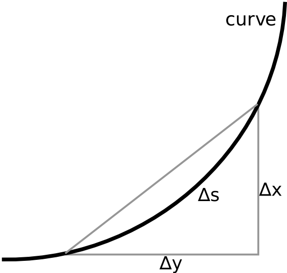
Approximating Deltas: For a small piece of curve, [latex]\Delta s[/latex] can be approximated with the Pythagorean theorem.
Surface Area
For rotations around the [latex]x[/latex]- and [latex]y[/latex]-axes, surface areas [latex]A_x[/latex] and [latex]A_y[/latex] are given, respectively, as the following: [latex-display]\displaystyle{A_x = \int 2\pi y \, ds, \,\, ds=\sqrt{1+\left(\frac{dy}{dx}\right)^2}dx \\ \\ A_y = \int 2\pi x \, ds, \,\, ds=\sqrt{1+\left(\frac{dx}{dy}\right)^2}dy }[/latex-display]Example
For a circle [latex]f(x) = \sqrt{1 -x^2}, 0 \leq x \leq 1[/latex], calculate the arc length. The curve can be represented parametrically as [latex]x=\sin(t), y=\cos(t)[/latex] for [latex]0 \leq t \leq \frac{\pi}{2}[/latex]. Therefore: [latex-display]\displaystyle{s = \int_0^{\frac{\pi}{2}}\sqrt{\cos^2(t)+\sin^2(t)} = \frac{\pi}{2}}[/latex-display] Now, calculate the surface area of the solid obtained by rotating [latex]f(x)[/latex] around the [latex]x[/latex]-axis: [latex-display]\displaystyle{A_x = \int_{0}^{1} 2\pi \sqrt{1-x^2}\cdot \sqrt{1+\left(\frac{-x}{\sqrt{1-x^2}}\right)^2} \, dx = 2\pi}[/latex-display]Area of a Surface of Revolution
If the curve is described by the function [latex]y = f(x) (a≤x≤b)[/latex], the area [latex]A_y[/latex] is given by the integral [latex]A_x = 2\pi\int_a^bf(x)\sqrt{1+\left(f'(x)\right)^2} \, dx[/latex] for revolution around the [latex]x[/latex]-axis.Learning Objectives
Use integration to find the area of a surface of revolutionKey Takeaways
Key Points
- A surface of revolution is a surface in Euclidean space created by rotating a curve around a straight line in its plane, known as the axis.
- If the curve is described by the parametric functions [latex]x(t)[/latex], [latex]y(t)[/latex], with [latex]t[/latex] ranging over some interval [latex][a,b][/latex] and the axis of revolution the [latex]y[/latex]-axis, then the area [latex]A_y[/latex] is given by the integral [latex]A_y = 2 \pi \int_a^b x(t) \ \sqrt{\left({dx \over dt}\right)^2 + \left({dy \over dt}\right)^2} \, dt[/latex].
- If the curve is described by the function [latex]y = f(x), a \leq x \leq b[/latex], then the integral becomes [latex]A_x = 2\pi\int_a^bf(x)\sqrt{1+\left(f'(x)\right)^2} \, dx[/latex] for revolution around the [latex]x[/latex]-axis.
- Examples of surfaces generated by a straight line are cylindrical and conical surfaces when the line is co-planar with the axis.
Key Terms
- torus: the standard representation of such a space in three-dimensional Euclidean space; a shape consisting of a ring with a circular cross-section; the shape of an inner tube or hollow doughnut
- euclidean space: ordinary two- or three-dimensional space (and higher dimensional generalizations), characterized by an infinite extent along each dimension and a constant distance between any pair of parallel lines
- revolution: rotation: the turning of an object around an axis
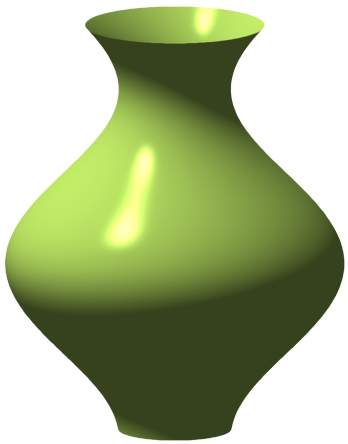
Surface of Revolution: A portion of the curve [latex]x=2+\cos z[/latex] rotated around the [latex]z[/latex]-axis (vertical in the figure).
Example
The spherical surface with a radius [latex]r[/latex] is generated by the curve [latex]x(t) =r \sin(t)[/latex], [latex]y(t) = r \cos(t)[/latex], when [latex]t[/latex] ranges over [latex][0,\pi][/latex]. Its area is therefore: [latex-display]\begin{align} A &{}= 2 \pi \int_0^\pi r\sin(t) \sqrt{\left(r\cos(t)\right)^2 + \left(r\sin(t)\right)^2} \, dt \\ &{}= 2 \pi r^2 \int_0^\pi \sin(t) \, dt \\ &{}= 4\pi r^2 \end{align}[/latex-display]Physics and Engineering: Fluid Pressure and Force
Pressure is given as [latex]p = \frac{F}{A}[/latex] or [latex]p = \frac{dF_n}{dA}[/latex], where [latex]p[/latex] is the pressure, [latex]\mathbf{F}[/latex] is the normal force, and [latex]A[/latex] is the area of the surface on contact.Learning Objectives
Apply the ideas of integration to pressureKey Takeaways
Key Points
- The pressure is the scalar proportionality constant that relates the two normal vectors [latex]d\mathbf{F}_n=-p\,d\mathbf{A} = -p\,\mathbf{n}\,dA[/latex].
- For fluids near the surface of the earth, the formula may be written as [latex]p = \rho g h[/latex], where [latex]p[/latex] is the pressure, [latex]\rho[/latex] is the density of the fluid, [latex]g[/latex] is the gravitational acceleration, and [latex]h[/latex] is the depth of the liquid in meters.
- Total force that the fluid pressure gives rise to is calculated as [latex]\mathbf{F_n} = -(\int \rho g h \, dA) \, \mathbf{n}[/latex].
Key Terms
- fluid: any substance which can flow with relative ease, tends to assume the shape of its container, and obeys Bernoulli's principle; a liquid, gas, or plasma
- Gravitational acceleration: acceleration on an object caused by gravity; at different points on Earth, an acceleration between 9.78 and 9.82 m/s2, depending on altitude
- Pressure: the amount of force that is applied over a given area divided by the size of this area

Fluid Pressure and Force: Pressure as exerted by particle collisions inside a closed container.
Physics and Engeineering: Center of Mass
For a continuous mass distribution, the position of center of mass is given as [latex]\mathbf R = \frac 1M \int_V\rho(\mathbf{r}) \mathbf{r} dV[/latex].Learning Objectives
Apply the ideas of integration to the center of massKey Takeaways
Key Points
- In physics, the center of mass (COM) of a distribution of mass in space is the unique point at which the weighted relative position of the distributed mass sums to zero.
- In the case of a system of particles Pi, i = 1, , n , each with mass, mi, which are located in space with coordinates ri, i = 1, , n, the coordinates R of the center of mass is [latex]\mathbf{R} = \frac{1}{M} \sum_{i=1}^n m_i \mathbf{r}_i[/latex].
- If the mass distribution is continuous with respect to the density, ρ(r), within a volume, V, then it follows that [latex]\mathbf R = \frac 1M \int_V\rho(\mathbf{r}) \mathbf{r} dV[/latex].
Key Terms
- centroid: the point at the center of any shape, sometimes called the center of area or the center of volume
Center of Mass
In physics, the center of mass (COM) of a mass or object in space is the unique point at which the weighted relative position of the distributed mass sums to zero. In this case, the distribution of mass is balanced around the center of mass and the average of the weighted position coordinates of the distributed mass defines its coordinates. Calculations in mechanics are simplified when formulated with respect to the COM.System of Particles
In the case of a system of particles [latex]P_i, i = 1, \cdots, n[/latex], each with a mass, [latex]m_i[/latex], which are located in space with coordinates [latex]r_i, i = 1, \cdots, n[/latex], the coordinates [latex]\mathbf{R}[/latex] of the center of mass satisfy the following condition: [latex-display]\displaystyle{\sum_{i=1}^n m_i(\mathbf{r}_i - \mathbf{R}) = 0}[/latex-display] Solve this equation for [latex]\mathbf{R}[/latex] to obtain the formula [latex-display]\displaystyle{\mathbf{R} = \frac{1}{M} \sum_{i=1}^n m_i \mathbf{r}_i}[/latex-display] where [latex]M[/latex] is the sum of the masses of all of the particles.Continuous Distribution
If the mass distribution is continuous with respect to the density, [latex]\rho (r)[/latex], within a volume, [latex]V[/latex], then the integral of the weighted position coordinates of the points in this volume relative to the center of mass, [latex]\mathbf{R}[/latex], is zero, that is: [latex-display]\displaystyle{\int_V \rho(\mathbf{r})(\mathbf{r}-\mathbf{R})dV = 0}[/latex-display] Solve this equation for the coordinates [latex]\mathbf{R}[/latex] to obtain: [latex-display]\displaystyle{\mathbf R = \frac 1M \int_V\rho(\mathbf{r}) \mathbf{r} dV}[/latex-display] where [latex]M[/latex] is the total mass in the volume. If a continuous mass distribution has uniform density, which means [latex]\rho[/latex] is constant, then the center of mass is the same as the centroid of the volume.
Two Bodies and the COM: Two bodies orbiting the COM located inside one body. COM can be defined for both discrete and continuous systems. The two objects are rotating around their center of mass.
Applications to Economics and Biology
Calculus has broad applications in diverse fields of science; examples of integration can be found in economics and biology.Learning Objectives
Apply the ideas behind integration to economics and biologyKey Takeaways
Key Points
- Consumer surplus is thus the definite integral of the demand function with respect to price, from the market price to the maximum reservation price [latex]CS = \int^{P_{\mathit{max}}}_{P_{\mathit{mkt}}} D(P)\, dP[/latex].
- The total flux of blood through a vessel with a radius [latex]R[/latex] can be expressed as [latex]F = \int_{0}^{R} 2\pi r \, v(r) \, dr[/latex], where [latex]v(r)[/latex] is the velocity of blood at [latex]r[/latex].
- Calculus, in general, has broad applications in diverse fields of science.
Key Terms
- flux: the rate of transfer of energy (or another physical quantity) through a given surface, specifically electric flux, magnetic flux
- cardiovascular: Relating to the circulatory system, that is the heart and blood vessels.
- surplus: specifically, an amount in the public treasury at any time greater than is required for the ordinary purposes of the government
Consumer Surplus
In mainstream economics, economic surplus (also known as total welfare or Marshallian surplus) refers to two related quantities. Consumer surplus is the monetary gain obtained by consumers; they are able to buy something for less than they had planned on spending. Producer surplus is the amount that producers benefit from selling at a market price that is higher than their lowest price, thereby making more profit.
Supply and Demand Chart: Graph illustrating consumer (red) and producer (blue) surpluses on a supply and demand chart.
Blood Flow
The human body is made up of several processes, all carrying out various functions, one of which is the continuous running of blood in the cardiovascular system. If we wanted, we could obtain a general expression for the volume of blood across a cross section per unit time (a quantity called flux). Since we can assume that there is a cylindrical symmetry in the blood vessel, we first consider the volume of blood passing through a ring with inner radius [latex]r[/latex] and outer radius [latex]r+dr[/latex] per unit time ([latex]dF[/latex]): [latex-display]dF = (2\pi r \, dr)\, v(r)[/latex-display] where [latex]v(r)[/latex] is the speed of blood at radius [latex]r[/latex]. Here, [latex]2 \pi r \,dr[/latex] is the area of the ring. Therefore, the total flux [latex]F[/latex] is written as: [latex-display]\displaystyle{F = \int_{0}^{R} 2\pi r \, v(r) \, dr}[/latex-display] where [latex]R[/latex] is the radius of the blood vessel. Once we have an (approximate) expression for [latex]v(r)[/latex], we can calculate the flux from the integral.
Blood Flow: (a) A tube; (b) The blood flow close to the edge of the tube is slower than that near the center.
Probability
Probability density function describes the relative likelihood, or probability, that a given variable will take on a value.Learning Objectives
Apply the ideas of integration to probability functions used in statisticsKey Takeaways
Key Points
- The probability of [latex]X[/latex] to be in a range [latex][a,b][/latex] is given as [latex]P [a \leq X \leq b] = \int_a^b f(x) \, \mathrm{d}x[/latex], where [latex]f(x) [/latex] is the probability density function in this case.
- The integral of the partial distribution function over the entire range of the variable is 1.
- The standard normal distribution has probability density [latex]f(X;\mu,\sigma^2) = \frac{1}{\sigma\sqrt{2\pi}} e^{ -\frac{1}{2}\left(\frac{X-\mu}{\sigma}\right)^2 }[/latex].
Key Terms
- probability density function: any function whose integral over a set gives the probability that a random variable has a value in that set
Probability Density Function
A probability density function is most commonly associated with absolutely continuous univariate distributions. For a continuous random variable [latex]X[/latex], the probability of [latex]X[/latex] to be in a range [latex][a,b][/latex] is given as: [latex-display]\displaystyle{P [a \leq X \leq b] = \int_a^b f(x) \, \mathrm{d}x}[/latex-display] where [latex]f(x)[/latex] is the probability density function in this case. The integral of the pdf in the range [latex][-\infty, \infty][/latex] is [latex-display]\displaystyle{\int_{-\infty}^{\infty} f(x) \, \mathrm{d}x \, = \, 1}[/latex-display] The expected value of [latex]X[/latex] (if it exists) can be calculated as: [latex-display]\displaystyle{E[X] = \int_{-\infty}^\infty x\,f(x)\,dx}[/latex-display]Example: Normal Distribution

Probability Distribution Function: Probability distribution function of a normal (or Gaussian) distribution, where mean [latex]\mu=0 [/latex] and variance [latex]\sigma^2=1[/latex].
Taylor Polynomials
A Taylor series is a representation of a function as an infinite sum of terms calculated from the values of the function's derivatives.Learning Objectives
Use the Taylor series to approximate an integralKey Takeaways
Key Points
- The Taylor series of a real or complex-valued function [latex]f(x)[/latex] that is infinitely differentiable in a neighborhood of a real or complex number a is the power series [latex]f(x) = \sum_{n=0} ^ {\infty} \frac {f^{(n)}(a)}{n! } \, (x-a)^{n}[/latex].
- Any finite number of initial terms of the Taylor series of a function is called a Taylor polynomial.
- Taylor series can be used to evaluate an integral when there is no other integration technique available (other than numerical integration).
Key Terms
- series: the sum of the terms of a sequence
- polynomial: an expression consisting of a sum of a finite number of terms, each term being the product of a constant coefficient and one or more variables raised to a non-negative integer power
Exponential Function as a Taylor Series: The exponential function (in blue) and the sum of the first 9 terms of its Taylor series at 0 (in red).
Example
The Taylor series for the exponential function [latex]e^x[/latex] at [latex]a=0[/latex] is: [latex-display]\displaystyle{e^x = \sum_{n=0}^{\infty} \frac{x^n}{n! } = 1 + \frac{x^1}{1! } + \frac{x^2}{2! } + \frac{x^3}{3! } + \cdots}[/latex-display]Using Taylor Series to Evaluate an Integral
Taylor series can be used to evaluate an integral when there is no other integration technique available (of course, other than numerical integration). Let's assume that the integration of a function ([latex]f(x)[/latex]) cannot be performed analytically. To evaluate the integral [latex]I = \int_{a}^{b} f(x) \, dx[/latex], we can Taylor-expand [latex]f(x)[/latex] and perform integration on individual terms of the series. Since [latex]f(x) = \sum_{n=0} ^ {\infty} \frac {f^{(n)}(0)}{n! } \, x^{n}[/latex], we get: [latex-display]\displaystyle{I = \sum_{n=0} ^ {\infty} \frac {f^{(n)}(0)}{n! } \, \int_{a}^{b}x^{n}\, dx \\ \, \,= \sum_{n=0} ^ {\infty} \frac {f^{(n)}(0)}{(n+1)! } \, (b^{n+1}-a^{n+1})}[/latex-display] Therefore, as long as Taylor expansion is possible and the infinite sum converges, the definite integral ([latex]I[/latex]) can be evaluated.Licenses & Attributions
CC licensed content, Shared previously
- Curation and Revision. Provided by: Boundless.com License: CC BY-SA: Attribution-ShareAlike.
CC licensed content, Specific attribution
- Arc length. Provided by: Wikipedia Located at: https://en.wikipedia.org/wiki/Arc_length. License: CC BY-SA: Attribution-ShareAlike.
- curve. Provided by: Wiktionary License: CC BY-SA: Attribution-ShareAlike.
- surface area. Provided by: Wiktionary License: CC BY-SA: Attribution-ShareAlike.
- Arc length. Provided by: Wikipedia License: CC BY: Attribution.
- Surface of revolution. Provided by: Wikipedia License: CC BY-SA: Attribution-ShareAlike.
- torus. Provided by: Wiktionary License: CC BY-SA: Attribution-ShareAlike.
- revolution. Provided by: Wiktionary License: CC BY-SA: Attribution-ShareAlike.
- euclidean space. Provided by: Wikipedia License: CC BY-SA: Attribution-ShareAlike.
- Arc length. Provided by: Wikipedia License: CC BY: Attribution.
- Surface of revolution. Provided by: Wikipedia License: CC BY: Attribution.
- Pressure. Provided by: Wikipedia License: CC BY-SA: Attribution-ShareAlike.
- Gravitational acceleration. Provided by: Wikipedia License: CC BY-SA: Attribution-ShareAlike.
- Pressure. Provided by: Wiktionary License: CC BY-SA: Attribution-ShareAlike.
- fluid. Provided by: Wiktionary License: CC BY-SA: Attribution-ShareAlike.
- Arc length. Provided by: Wikipedia License: CC BY: Attribution.
- Surface of revolution. Provided by: Wikipedia License: CC BY: Attribution.
- Pressure. Provided by: Wikipedia License: CC BY: Attribution.
- Center of mass. Provided by: Wikipedia License: CC BY-SA: Attribution-ShareAlike.
- centroid. Provided by: Wiktionary License: CC BY-SA: Attribution-ShareAlike.
- Arc length. Provided by: Wikipedia License: CC BY: Attribution.
- Surface of revolution. Provided by: Wikipedia License: CC BY: Attribution.
- Pressure. Provided by: Wikipedia License: CC BY: Attribution.
- Center of mass. Provided by: Wikipedia License: CC BY: Attribution.
- Economic surplus. Provided by: Wikipedia License: CC BY-SA: Attribution-ShareAlike.
- Blood flow. Provided by: Wikipedia License: CC BY-SA: Attribution-ShareAlike.
- Economic surplus. Provided by: Wikipedia License: CC BY-SA: Attribution-ShareAlike.
- flux. Provided by: Wiktionary License: CC BY-SA: Attribution-ShareAlike.
- cardiovascular. Provided by: Wiktionary License: CC BY-SA: Attribution-ShareAlike.
- surplus. Provided by: Wiktionary License: CC BY-SA: Attribution-ShareAlike.
- Arc length. Provided by: Wikipedia License: CC BY: Attribution.
- Surface of revolution. Provided by: Wikipedia License: CC BY: Attribution.
- Pressure. Provided by: Wikipedia License: CC BY: Attribution.
- Center of mass. Provided by: Wikipedia License: CC BY: Attribution.
- Economic surplus. Provided by: Wikipedia License: CC BY: Attribution.
- Hagenu2013Poiseuille equation. Provided by: Wikipedia License: CC BY: Attribution.
- Normal distribution. Provided by: Wikipedia License: CC BY-SA: Attribution-ShareAlike.
- Probability density function. Provided by: Wikipedia License: CC BY-SA: Attribution-ShareAlike.
- probability density function. Provided by: Wiktionary Located at: https://en.wiktionary.org/wiki/probability_density_function. License: CC BY-SA: Attribution-ShareAlike.
- Arc length. Provided by: Wikipedia License: CC BY: Attribution.
- Surface of revolution. Provided by: Wikipedia License: CC BY: Attribution.
- Pressure. Provided by: Wikipedia License: CC BY: Attribution.
- Center of mass. Provided by: Wikipedia License: CC BY: Attribution.
- Economic surplus. Provided by: Wikipedia License: CC BY: Attribution.
- Hagenu2013Poiseuille equation. Provided by: Wikipedia License: CC BY: Attribution.
- Normal distribution. Provided by: Wikipedia License: CC BY: Attribution.
- series. Provided by: Wiktionary License: CC BY-SA: Attribution-ShareAlike.
- Taylor series. Provided by: Wikipedia License: CC BY-SA: Attribution-ShareAlike.
- polynomial. Provided by: Wiktionary License: CC BY-SA: Attribution-ShareAlike.
- Arc length. Provided by: Wikipedia License: CC BY: Attribution.
- Surface of revolution. Provided by: Wikipedia License: CC BY: Attribution.
- Pressure. Provided by: Wikipedia License: CC BY: Attribution.
- Center of mass. Provided by: Wikipedia License: CC BY: Attribution.
- Economic surplus. Provided by: Wikipedia License: CC BY: Attribution.
- Hagenu2013Poiseuille equation. Provided by: Wikipedia License: CC BY: Attribution.
- Normal distribution. Provided by: Wikipedia License: CC BY: Attribution.
- Taylor series. Provided by: Wikipedia License: CC BY: Attribution.
