
Equations of Exponential Functions
Learning Outcomes
- Given two data points, write an exponential function.
- Identify initial conditions for an exponential function.
- Find an exponential function given a graph.
- Use a graphing calculator to find an exponential function.
- Find an exponential function that models continuous growth or decay.
tip for success
When writing an exponential model from two data points, recall the processes you've learned to write other types of models from data points contained on the graphs of linear, power, polynomial, and rational functions. Each process was different, but each followed a fundamental characteristic of functions: that every point on the graph of a function satisfies the equation of the function. The process of writing an exponential model capitalizes on the same idea. See the examples below for how to write an exponential model.How To: Given two data points, write an exponential model
- If one of the data points has the form [latex]\left(0,a\right)[/latex], then a is the initial value. Using a, substitute the second point into the equation [latex]f\left(x\right)=a{b}^{x}[/latex], and solve for b.
- If neither of the data points have the form [latex]\left(0,a\right)[/latex], substitute both points into two equations with the form [latex]f\left(x\right)=a{b}^{x}[/latex]. Solve the resulting system of two equations to find [latex]a[/latex] and [latex]b[/latex].
- Using the a and b found in the steps above, write the exponential function in the form [latex]f\left(x\right)=a{b}^{x}[/latex].
Example: Writing an Exponential Model When the Initial Value Is Known
In 2006, 80 deer were introduced into a wildlife refuge. By 2012, the population had grown to 180 deer. The population was growing exponentially. Write an algebraic function N(t) representing the population N of deer over time t.Answer: We let our independent variable t be the number of years after 2006. Thus, the information given in the problem can be written as input-output pairs: (0, 80) and (6, 180). Notice that by choosing our input variable to be measured as years after 2006, we have given ourselves the initial value for the function, a = 80. We can now substitute the second point into the equation [latex]N\left(t\right)=80{b}^{t}[/latex] to find b:
[latex]\begin{array}{c}N\left(t\right)\hfill & =80{b}^{t}\hfill & \hfill \\ 180\hfill & =80{b}^{6}\hfill & \text{Substitute using point }\left(6, 180\right).\hfill \\ \frac{9}{4}\hfill & ={b}^{6}\hfill & \text{Divide and write in lowest terms}.\hfill \\ b\hfill & ={\left(\frac{9}{4}\right)}^{\frac{1}{6}}\hfill & \text{Isolate }b\text{ using properties of exponents}.\hfill \\ b\hfill & \approx 1.1447 & \text{Round to 4 decimal places}.\hfill \end{array}[/latex]
NOTE: Unless otherwise stated, do not round any intermediate calculations. Round the final answer to four places for the remainder of this section. The exponential model for the population of deer is [latex]N\left(t\right)=80{\left(1.1447\right)}^{t}[/latex]. Note that this exponential function models short-term growth. As the inputs get larger, the outputs will get increasingly larger resulting in the model not being useful in the long term due to extremely large output values. We can graph our model to observe the population growth of deer in the refuge over time. Notice that the graph below passes through the initial points given in the problem, [latex]\left(0,\text{ 8}0\right)[/latex] and [latex]\left(\text{6},\text{ 18}0\right)[/latex]. We can also see that the domain for the function is [latex]\left[0,\infty \right)[/latex] and the range for the function is [latex]\left[80,\infty \right)[/latex]. Graph showing the population of deer over time, [latex]N\left(t\right)=80{\left(1.1447\right)}^{t}[/latex], t years after 2006
Try It
A wolf population is growing exponentially. In 2011, 129 wolves were counted. By 2013 the population had reached 236 wolves. What two points can be used to derive an exponential equation modeling this situation? Write the equation representing the population N of wolves over time t.Answer: [latex]\left(0,129\right)[/latex] and [latex]\left(2,236\right);N\left(t\right)=129{\left(\text{1}\text{.3526}\right)}^{t}[/latex]
Example: Writing an Exponential Model When the Initial Value is Not Known
Find an exponential function that passes through the points [latex]\left(-2,6\right)[/latex] and [latex]\left(2,1\right)[/latex].Answer: Because we don’t have the initial value, we substitute both points into an equation of the form [latex]f\left(x\right)=a{b}^{x}[/latex] and then solve the system for a and b.
- Substituting [latex]\left(-2,6\right)[/latex] gives [latex]6=a{b}^{-2}[/latex]
- Substituting [latex]\left(2,1\right)[/latex] gives [latex]1=a{b}^{2}[/latex]
[latex]\begin{array}{l}6=ab^{-2}\\\frac{6}{b^{-2}}=a\,\,\,\,\,\,\,\,\text{Divide.}\\a=6b^{2}\,\,\,\,\,\,\,\,\text{Use properties of exponents to rewrite the denominator.}\end{array}[/latex]
Substitute a in the second equation and solve for b:[latex]\begin{array}{l}1=ab^{2}\\1=6b^{2}b^{2}=6b^{4}\,\,\,\,\,\text{Substitute }a.\\b=\left(\frac{1}{6}\right)^{\frac{1}{4}}\,\,\,\,\,\,\,\,\,\,\,\,\,\,\,\,\,\,\,\text{Use properties of exponents to isolate }b.\\b\approx0.6389\,\,\,\,\,\,\,\,\,\,\,\,\,\,\,\,\,\,\text{Round 4 decimal places.}\end{array}[/latex]
Use the value of b in the first equation to solve for the value of a:[latex]a=6b^{2}\approx6\left(0.6389\right)^{2}\approx2.4492[/latex]
Thus, the equation is [latex]f\left(x\right)=2.4492{\left(0.6389\right)}^{x}[/latex]. We can graph our model to check our work. Notice that the graph below passes through the initial points given in the problem, [latex]\left(-2,\text{ 6}\right)[/latex] and [latex]\left(2,\text{ 1}\right)[/latex]. The graph is an example of an exponential decay function. The graph of [latex]f\left(x\right)=2.4492{\left(0.6389\right)}^{x}[/latex] models exponential decay.
Try It
Given the two points [latex]\left(1,3\right)[/latex] and [latex]\left(2,4.5\right)[/latex], find the equation of the exponential function that passes through these two points.Answer: [latex]f\left(x\right)=2{\left(1.5\right)}^{x}[/latex]
[ohm_question]2942[/ohm_question]Q & A
Do two points always determine a unique exponential function? Yes, provided the two points are either both above the x-axis or both below the x-axis and have different x-coordinates. But keep in mind that we also need to know that the graph is, in fact, an exponential function. Not every graph that looks exponential really is exponential. We need to know the graph is based on a model that shows the same percent growth with each unit increase in x, which in many real world cases involves time.How To: Given the graph of an exponential function, write its equation
- First, identify two points on the graph. Choose the y-intercept as one of the two points whenever possible. Try to choose points that are as far apart as possible to reduce round-off error.
- If one of the data points is the y-intercept [latex]\left(0,a\right)[/latex] , then a is the initial value. Using a, substitute the second point into the equation [latex]f\left(x\right)=a{b}^{x}[/latex] and solve for b.
- If neither of the data points have the form [latex]\left(0,a\right)[/latex], substitute both points into two equations with the form [latex]f\left(x\right)=a{b}^{x}[/latex]. Solve the resulting system of two equations to find a and b.
- Write the exponential function, [latex]f\left(x\right)=a{b}^{x}[/latex].
Example: Writing an Exponential Function Given Its Graph
Find an equation for the exponential function graphed below.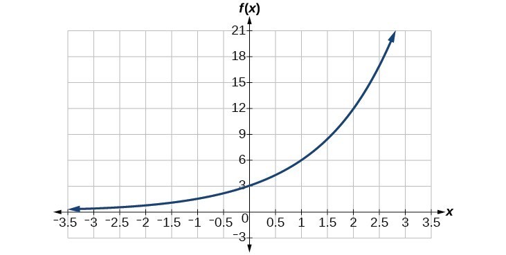
Answer: We can choose the y-intercept of the graph, [latex]\left(0,3\right)[/latex], as our first point. This gives us the initial value [latex]a=3[/latex]. Next, choose a point on the curve some distance away from [latex]\left(0,3\right)[/latex] that has integer coordinates. One such point is [latex]\left(2,12\right)[/latex].
[latex]\begin{array}{llllll}y=a{b}^{x}& \text{Write the general form of an exponential equation}. \\ y=3{b}^{x} & \text{Substitute the initial value 3 for }a. \\ 12=3{b}^{2} & \text{Substitute in 12 for }y\text{ and 2 for }x. \\ 4={b}^{2} & \text{Divide by 3}. \\ b=\pm 2 & \text{Take the square root}.\end{array}[/latex]
Because we restrict ourselves to positive values of b, we will use b = 2. Substitute a and b into standard form to yield the equation [latex]f\left(x\right)=3{\left(2\right)}^{x}[/latex].Try It
Find an equation for the exponential function graphed below.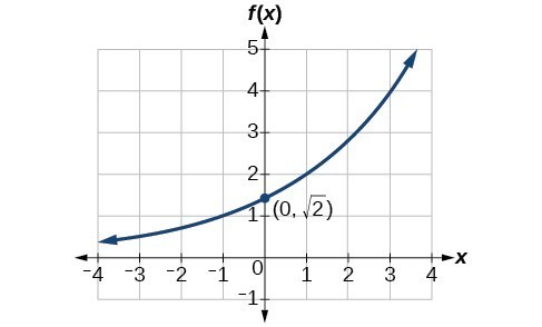
Answer: [latex]f\left(x\right)=\sqrt{2}{\left(\sqrt{2}\right)}^{x}[/latex]. Answers may vary due to round-off error. The answer should be very close to [latex]1.4142{\left(1.4142\right)}^{x}[/latex].
Investigating Continuous Growth
So far we have worked with rational bases for exponential functions. For most real-world phenomena, however, e is used as the base for exponential functions. Exponential models that use e as the base are called continuous growth or decay models. We see these models in finance, computer science, and most of the sciences such as physics, toxicology, and fluid dynamics.A General Note: The Continuous Growth/Decay Formula
For all real numbers t, and all positive numbers a and r, continuous growth or decay is represented by the formula[latex]A\left(t\right)=a{e}^{rt}[/latex]
where- a is the initial value
- r is the continuous growth rate per unit of time
- t is the elapsed time
[latex]A\left(t\right)=P{e}^{rt}[/latex]
where- P is the principal or the initial investment
- r is the growth or interest rate per unit of time
- t is the period or term of the investment
How To: Given the initial value, rate of growth or decay, and time t, solve a continuous growth or decay function
- Use the information in the problem to determine a, the initial value of the function.
- Use the information in the problem to determine the growth rate r.
- If the problem refers to continuous growth, then r > 0.
- If the problem refers to continuous decay, then r < 0.
- Use the information in the problem to determine the time t.
- Substitute the given information into the continuous growth formula and solve for A(t).
Example: Calculating Continuous Growth
A person invested $1,000 in an account earning a nominal interest rate of 10% per year compounded continuously. How much was in the account at the end of one year?Answer: Since the account is growing in value, this is a continuous compounding problem with growth rate r = 0.10. The initial investment was $1,000, so P = 1000. We use the continuous compounding formula to find the value after t = 1 year:
[latex]\begin{array}{c}A\left(t\right)\hfill & =P{e}^{rt}\hfill & \text{Use the continuous compounding formula}.\hfill \\ \hfill & =1000{\left(e\right)}^{0.1} & \text{Substitute known values for }P, r,\text{ and }t.\hfill \\ \hfill & \approx 1105.17\hfill & \text{Use a calculator to approximate}.\hfill \end{array}[/latex]
The account is worth $1,105.17 after one year.Try It
A person invests $100,000 at a nominal 12% interest per year compounded continuously. What will be the value of the investment in 30 years?Answer: $3,659,823.44
[ohm_question]25526[/ohm_question]Example: Calculating Continuous Decay
Radon-222 decays at a continuous rate of 17.3% per day. How much will 100 mg of Radon-[latex]222[/latex] decay to in [latex]3[/latex] days?Answer: Since the substance is decaying, the rate, [latex]17.3%[/latex], is negative. So, [latex]r=-0.173[/latex]. The initial amount of radon-[latex]222[/latex] was [latex]100[/latex] mg, so [latex]a= 100[/latex]. We use the continuous decay formula to find the value after [latex]t= 3[/latex] days:
[latex]\begin{array}{c}A\left(t\right)\hfill & =a{e}^{rt}\hfill & \text{Use the continuous growth formula}.\hfill \\ \hfill & =100{e}^{-0.173\left(3\right)} & \text{Substitute known values for }a, r,\text{ and }t.\hfill \\ \hfill & \approx 59.5115\hfill & \text{Use a calculator to approximate}.\hfill \end{array}[/latex]
So [latex]59.5115[/latex] mg of radon-[latex]222[/latex] will remain.Try It
Using the data in the previous example, how much radon-222 will remain after one year?Answer: [latex]3.77115984\small{E }-26[/latex] (This is calculator notation for the number written as [latex]3.77\times {10}^{-26}[/latex] in scientific notation. While the output of an exponential function is never zero, this number is so close to zero that for all practical purposes we can accept zero as the answer.)
Licenses & Attributions
CC licensed content, Original
- Revision and Adaptation. Provided by: Lumen Learning License: CC BY: Attribution.
CC licensed content, Shared previously
- Question ID 25526 . Authored by: Morales,Lawrence, mb Lippman,David, mb Sousa,James. License: CC BY: Attribution. License terms: IMathAS Community License CC-BY + GPL.
- College Algebra. Provided by: OpenStax Authored by: Abramson, Jay et al.. Located at: https://openstax.org/books/college-algebra/pages/1-introduction-to-prerequisites. License: CC BY: Attribution. License terms: Download for free at http://cnx.org/contents/[email protected].
- Question ID 2942. Authored by: Anderson,Tophe. License: CC BY: Attribution. License terms: IMathAS Community License CC-BY + GPL.
