
The Second Derivative Test and Curve Sketching
Learning Objectives
- Use concavity and inflection points to explain how the sign of the second derivative affects the shape of a function’s graph.
- Explain the concavity test for a function over an open interval.
- Explain the relationship between a function and its first and second derivatives.
- State the second derivative test for local extrema.
- Analyze a function and its derivatives to draw its graph.
Concavity and Points of Inflection
We now know how to determine where a function is increasing or decreasing. However, there is another issue to consider regarding the shape of the graph of a function. If the graph curves, does it curve upward or curve downward? This notion is called the concavity of the function.
(Figure)(a) shows a function [latex]f[/latex] with a graph that curves upward. As [latex]x[/latex] increases, the slope of the tangent line increases. Thus, since the derivative increases as [latex]x[/latex] increases, [latex]f^{\prime}[/latex] is an increasing function. We say this function [latex]f[/latex] is concave up. (Figure)(b) shows a function [latex]f[/latex] that curves downward. As [latex]x[/latex] increases, the slope of the tangent line decreases. Since the derivative decreases as [latex]x[/latex] increases, [latex]f^{\prime}[/latex] is a decreasing function. We say this function [latex]f[/latex] is concave down.
Definition
Let [latex]f[/latex] be a function that is differentiable over an open interval [latex]I[/latex]. If [latex]f^{\prime}[/latex] is increasing over [latex]I[/latex], we say [latex]f[/latex] is concave up over [latex]I[/latex]. If [latex]f^{\prime}[/latex] is decreasing over [latex]I[/latex], we say [latex]f[/latex] is concave down over [latex]I[/latex].
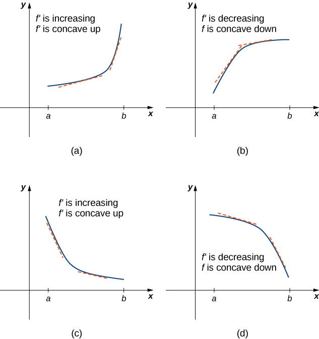 Figure 5. (a), (c) Since [latex]f^{\prime}[/latex] is increasing over the interval [latex](a,b)[/latex], we say [latex]f[/latex] is concave up over [latex](a,b)[/latex]. (b), (d) Since [latex]f^{\prime}[/latex] is decreasing over the interval [latex](a,b)[/latex], we say [latex]f[/latex] is concave down over [latex](a,b)[/latex].
In general, without having the graph of a function [latex]f[/latex], how can we determine its concavity? By definition, a function [latex]f[/latex] is concave up if [latex]f^{\prime}[/latex] is increasing. From Corollary 3, we know that if [latex]f^{\prime}[/latex] is a differentiable function, then [latex]f^{\prime}[/latex] is increasing if its derivative [latex]f^{\prime \prime}(x)>0[/latex]. Therefore, a function [latex]f[/latex] that is twice differentiable is concave up when [latex]f^{\prime \prime}(x)>0[/latex]. Similarly, a function [latex]f[/latex] is concave down if [latex]f^{\prime}[/latex] is decreasing. We know that a differentiable function [latex]f^{\prime}[/latex] is decreasing if its derivative [latex]f^{\prime \prime}(x)<0[/latex]. Therefore, a twice-differentiable function [latex]f[/latex] is concave down when [latex]f^{\prime \prime}(x)<0[/latex]. Applying this logic is known as the concavity test.
Test for Concavity
Let [latex]f[/latex] be a function that is twice differentiable over an interval [latex]I[/latex].
- If [latex]f^{\prime \prime}(x)>0[/latex] for all [latex]x \in I[/latex], then [latex]f[/latex] is concave up over [latex]I[/latex].
- If [latex]f^{\prime \prime}(x)<0[/latex] for all [latex]x \in I[/latex], then [latex]f[/latex] is concave down over [latex]I[/latex].
We conclude that we can determine the concavity of a function [latex]f[/latex] by looking at the second derivative of [latex]f[/latex]. In addition, we observe that a function [latex]f[/latex] can switch concavity ((Figure)). However, a continuous function can switch concavity only at a point [latex]x[/latex] if [latex]f^{\prime \prime}(x)=0[/latex] or [latex]f^{\prime \prime}(x)[/latex] is undefined. Consequently, to determine the intervals where a function [latex]f[/latex] is concave up and concave down, we look for those values of [latex]x[/latex] where [latex]f^{\prime \prime}(x)=0[/latex] or [latex]f^{\prime \prime}(x)[/latex] is undefined. When we have determined these points, we divide the domain of [latex]f[/latex] into smaller intervals and determine the sign of [latex]f^{\prime \prime}[/latex] over each of these smaller intervals. If [latex]f^{\prime \prime}[/latex] changes sign as we pass through a point [latex]x[/latex], then [latex]f[/latex] changes concavity. It is important to remember that a function [latex]f[/latex] may not change concavity at a point [latex]x[/latex] even if [latex]f^{\prime \prime}(x)=0[/latex] or [latex]f^{\prime \prime}(x)[/latex] is undefined. If, however, [latex]f[/latex] does change concavity at a point [latex]a[/latex] and [latex]f[/latex] is continuous at [latex]a[/latex], we say the point [latex](a,f(a))[/latex] is an inflection point of [latex]f[/latex].
Definition
If [latex]f[/latex] is continuous at [latex]a[/latex] and [latex]f[/latex] changes concavity at [latex]a[/latex], the point [latex](a,f(a))[/latex] is an inflection point of [latex]f[/latex].
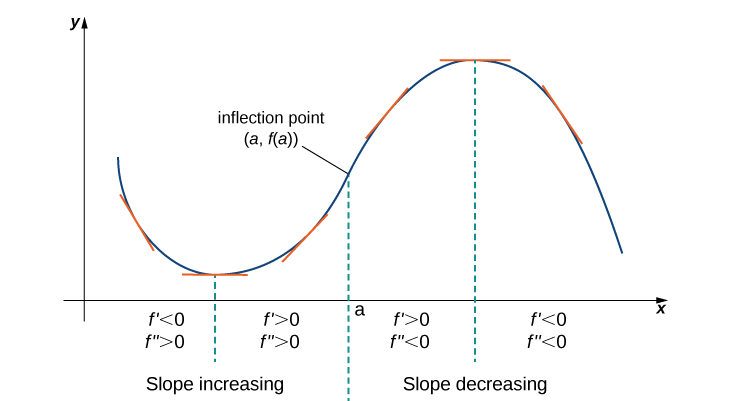 Figure 6. Since [latex]f^{\prime \prime}(x)>0[/latex] for [latex]x<a[/latex], the function [latex]f[/latex] is concave up over the interval [latex](−\infty,a)[/latex]. Since [latex]f^{\prime \prime}(x)<0[/latex] for [latex]x>a[/latex], the function [latex]f[/latex] is concave down over the interval [latex](a,\infty)[/latex]. The point [latex](a,f(a))[/latex] is an inflection point of [latex]f[/latex].
Testing for Concavity
For the function [latex]f(x)=x^3-6x^2+9x+30[/latex], determine all intervals where [latex]f[/latex] is concave up and all intervals where [latex]f[/latex] is concave down. List all inflection points for [latex]f[/latex]. Use a graphing utility to confirm your results.
Answer:
To determine concavity, we need to find the second derivative [latex]f^{\prime \prime}(x)[/latex]. The first derivative is [latex]f^{\prime}(x)=3x^2-12x+9[/latex], so the second derivative is [latex]f^{\prime \prime}(x)=6x-12[/latex]. If the function changes concavity, it occurs either when [latex]f^{\prime \prime}(x)=0[/latex] or [latex]f^{\prime \prime}(x)[/latex] is undefined. Since [latex]f^{\prime \prime}[/latex] is defined for all real numbers [latex]x[/latex], we need only find where [latex]f^{\prime \prime}(x)=0[/latex]. Solving the equation [latex]6x-12=0[/latex], we see that [latex]x=2[/latex] is the only place where [latex]f[/latex] could change concavity. We now test points over the intervals [latex](−\infty ,2)[/latex] and [latex](2,\infty)[/latex] to determine the concavity of [latex]f[/latex]. The points [latex]x=0[/latex] and [latex]x=3[/latex] are test points for these intervals.
| Interval | Test Point | Sign of [latex]f^{\prime \prime}(x)=6x-12[/latex] at Test Point | Conclusion |
|---|---|---|---|
| [latex](−\infty ,2)[/latex] | [latex]x=0[/latex] | [latex]-[/latex] | [latex]f[/latex] is concave down |
| [latex](2,\infty )[/latex] | [latex]x=3[/latex] | [latex]+[/latex] | [latex]f[/latex] is concave up. |
We conclude that [latex]f[/latex] is concave down over the interval [latex](−\infty ,2)[/latex] and concave up over the interval [latex](2,\infty)[/latex]. Since [latex]f[/latex] changes concavity at [latex]x=2[/latex], the point [latex](2,f(2))=(2,32)[/latex] is an inflection point. (Figure) confirms the analytical results.
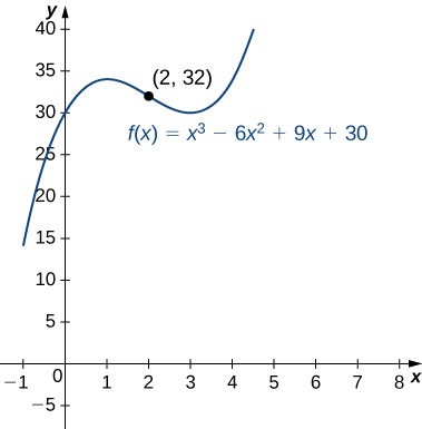 Figure 7. The given function has a point of inflection at [latex](2,32)[/latex] where the graph changes concavity.
For [latex]f(x)=−x^3+\frac{3}{2}x^2+18x[/latex], find all intervals where [latex]f[/latex] is concave up and all intervals where [latex]f[/latex] is concave down.
Answer:
[latex]f[/latex] is concave up over the interval [latex](−\infty ,\frac{1}{2})[/latex] and concave down over the interval [latex](\frac{1}{2},\infty )[/latex]
We now summarize, in (Figure), the information that the first and second derivatives of a function [latex]f[/latex] provide about the graph of [latex]f[/latex], and illustrate this information in (Figure).
| Sign of [latex]f^{\prime}[/latex] | Sign of [latex]f^{\prime \prime}[/latex] | Is [latex]f[/latex] increasing or decreasing? | Concavity |
|---|---|---|---|
| Positive | Positive | Increasing | Concave up |
| Positive | Negative | Increasing | Concave down |
| Negative | Positive | Decreasing | Concave up |
| Negative | Negative | Decreasing | Concave down |
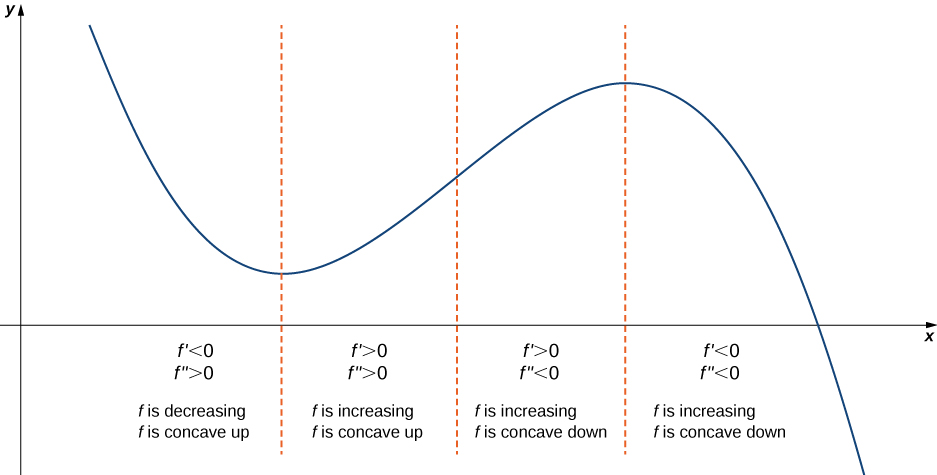 Figure 8. Consider a twice-differentiable function [latex]f[/latex] over an open interval [latex]I[/latex]. If [latex]f^{\prime}(x)>0[/latex] for all [latex]x \in I[/latex], the function is increasing over [latex]I[/latex]. If [latex]f^{\prime}(x)<0[/latex] for all [latex]x \in I[/latex], the function is decreasing over [latex]I[/latex]. If [latex]f^{\prime \prime}(x)>0[/latex] for all [latex]x \in I[/latex], the function is concave up. If [latex]f^{\prime \prime}(x)<0[/latex] for all [latex]x \in I[/latex], the function is concave down on [latex]I[/latex].
The Second Derivative Test
The first derivative test provides an analytical tool for finding local extrema, but the second derivative can also be used to locate extreme values. Using the second derivative can sometimes be a simpler method than using the first derivative.
We know that if a continuous function has a local extrema, it must occur at a critical point. However, a function need not have a local extrema at a critical point. Here we examine how the second derivative test can be used to determine whether a function has a local extremum at a critical point. Let [latex]f[/latex] be a twice-differentiable function such that [latex]f^{\prime}(a)=0[/latex] and [latex]f^{\prime \prime}[/latex] is continuous over an open interval [latex]I[/latex] containing [latex]a[/latex]. Suppose [latex]f^{\prime \prime}(a)<0[/latex]. Since [latex]f^{\prime \prime}[/latex] is continuous over [latex]I[/latex], [latex]f^{\prime \prime}(x)<0[/latex] for all [latex]x \in I[/latex] ((Figure)). Then, by Corollary 3, [latex]f^{\prime}[/latex] is a decreasing function over [latex]I[/latex]. Since [latex]f^{\prime}(a)=0[/latex], we conclude that for all [latex]x \in I, \, f^{\prime}(x)>0[/latex] if [latex]x<a[/latex] and [latex]f^{\prime}(x)<0[/latex] if [latex]x>a[/latex]. Therefore, by the first derivative test, [latex]f[/latex] has a local maximum at [latex]x=a[/latex]. On the other hand, suppose there exists a point [latex]b[/latex] such that [latex]f^{\prime}(b)=0[/latex] but [latex]f^{\prime \prime}(b)>0[/latex]. Since [latex]f^{\prime \prime}[/latex] is continuous over an open interval [latex]I[/latex] containing [latex]b[/latex], then [latex]f^{\prime \prime}(x)>0[/latex] for all [latex]x \in I[/latex] ((Figure)). Then, by Corollary [latex]3, \, f^{\prime}[/latex] is an increasing function over [latex]I[/latex]. Since [latex]f^{\prime}(b)=0[/latex], we conclude that for all [latex]x \in I[/latex], [latex]f^{\prime}(x)<0[/latex] if [latex]x<b[/latex] and [latex]f^{\prime}(x)>0[/latex] if [latex]x>b[/latex]. Therefore, by the first derivative test, [latex]f[/latex] has a local minimum at [latex]x=b[/latex].
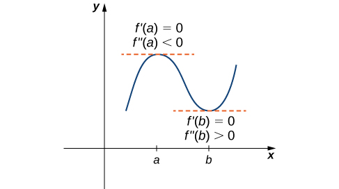 Figure 9. Consider a twice-differentiable function [latex]f[/latex] such that [latex]f^{\prime \prime}[/latex] is continuous. Since [latex]f^{\prime}(a)=0[/latex] and [latex]f^{\prime \prime}(a)<0[/latex], there is an interval [latex]I[/latex] containing [latex]a[/latex] such that for all [latex]x[/latex] in [latex]I[/latex], [latex]f[/latex] is increasing if [latex]x<a[/latex] and [latex]f[/latex] is decreasing if [latex]x>a[/latex]. As a result, [latex]f[/latex] has a local maximum at [latex]x=a[/latex]. Since [latex]f^{\prime}(b)=0[/latex] and [latex]f^{\prime \prime}(b)>0[/latex], there is an interval [latex]I[/latex] containing [latex]b[/latex] such that for all [latex]x[/latex] in [latex]I[/latex], [latex]f[/latex] is decreasing if [latex]x<b[/latex] and [latex]f[/latex] is increasing if [latex]x>b[/latex]. As a result, [latex]f[/latex] has a local minimum at [latex]x=b[/latex].
Second Derivative Test
Suppose [latex]f^{\prime}(c)=0, \, f^{\prime \prime}[/latex] is continuous over an interval containing [latex]c[/latex].
- If [latex]f^{\prime \prime}(c)>0[/latex], then [latex]f[/latex] has a local minimum at [latex]c[/latex].
- If [latex]f^{\prime \prime}(c)<0[/latex], then [latex]f[/latex] has a local maximum at [latex]c[/latex].
- If [latex]f^{\prime \prime}(c)=0[/latex], then the test is inconclusive.
Note that for case iii. when [latex]f^{\prime \prime}(c)=0[/latex], then [latex]f[/latex] may have a local maximum, local minimum, or neither at [latex]c[/latex]. For example, the functions [latex]f(x)=x^3[/latex], [latex]f(x)=x^4[/latex], and [latex]f(x)=−x^4[/latex] all have critical points at [latex]x=0[/latex]. In each case, the second derivative is zero at [latex]x=0[/latex]. However, the function [latex]f(x)=x^4[/latex] has a local minimum at [latex]x=0[/latex] whereas the function [latex]f(x)=−x^4[/latex] has a local maximum at [latex]x=0[/latex] and the function [latex]f(x)=x^3[/latex] does not have a local extremum at [latex]x=0[/latex].
Let’s now look at how to use the second derivative test to determine whether [latex]f[/latex] has a local maximum or local minimum at a critical point [latex]c[/latex] where [latex]f^{\prime}(c)=0[/latex].
Using the Second Derivative Test
Use the second derivative to find the location of all local extrema for [latex]f(x)=x^5-5x^3[/latex].
Answer:
To apply the second derivative test, we first need to find critical points [latex]c[/latex] where [latex]f^{\prime}(c)=0[/latex]. The derivative is [latex]f^{\prime}(x)=5x^4-15x^2[/latex]. Therefore, [latex]f^{\prime}(x)=5x^4-15x^2=5x^2(x^2-3)=0[/latex] when [latex]x=0,\pm \sqrt{3}[/latex].
To determine whether [latex]f[/latex] has a local extrema at any of these points, we need to evaluate the sign of [latex]f^{\prime \prime}[/latex] at these points. The second derivative is
In the following table, we evaluate the second derivative at each of the critical points and use the second derivative test to determine whether [latex]f[/latex] has a local maximum or local minimum at any of these points.
| [latex]x[/latex] | [latex]f^{\prime \prime}(x)[/latex] | Conclusion |
|---|---|---|
| [latex]−\sqrt{3}[/latex] | [latex]-30\sqrt{3}[/latex] | Local maximum |
| 0 | 0 | Second derivative test is inconclusive |
| [latex]\sqrt{3}[/latex] | [latex]30\sqrt{3}[/latex] | Local minimum |
By the second derivative test, we conclude that [latex]f[/latex] has a local maximum at [latex]x=−\sqrt{3}[/latex] and [latex]f[/latex] has a local minimum at [latex]x=\sqrt{3}[/latex]. The second derivative test is inconclusive at [latex]x=0[/latex]. To determine whether [latex]f[/latex] has a local extrema at [latex]x=0[/latex], we apply the first derivative test. To evaluate the sign of [latex]f^{\prime}(x)=5x^2(x^2-3)[/latex] for [latex]x \in (−\sqrt{3},0)[/latex] and [latex]x \in (0,\sqrt{3})[/latex], let [latex]x=-1[/latex] and [latex]x=1[/latex] be the two test points. Since [latex]f^{\prime}(-1)<0[/latex] and [latex]f^{\prime}(1)<0[/latex], we conclude that [latex]f[/latex] is decreasing on both intervals and, therefore, [latex]f[/latex] does not have a local extrema at [latex]x=0[/latex] as shown in the following graph.
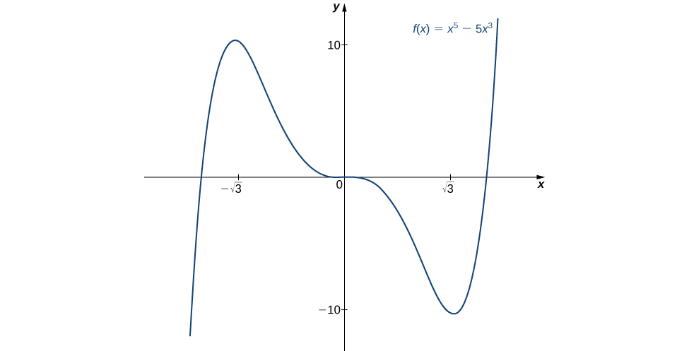 Figure 10. The function [latex]f[/latex] has a local maximum at [latex]x=−\sqrt{3}[/latex] and a local minimum at [latex]x=\sqrt{3}[/latex]
Consider the function [latex]f(x)=x^3-(\frac{3}{2})x^2-18x[/latex]. The points [latex]c=3,-2[/latex] satisfy [latex]f^{\prime}(c)=0[/latex]. Use the second derivative test to determine whether [latex]f[/latex] has a local maximum or local minimum at those points.
Answer:
[latex]f[/latex] has a local maximum at -2 and a local minimum at 3.
Hint
[latex]f^{\prime \prime}(x)=6x-3[/latex]
We have now developed the tools we need to determine where a function is increasing and decreasing, as well as acquired an understanding of the basic shape of the graph. Next we discuss what happens to a function as [latex]x \to \pm \infty[/latex]. At that point, we have enough tools to provide accurate graphs of a large variety of functions.
Guidelines for Drawing the Graph of a Function
We now have enough analytical tools to draw graphs of a wide variety of algebraic and transcendental functions. Before showing how to graph specific functions, let’s look at a general strategy to use when graphing any function.
Problem-Solving Strategy: Drawing the Graph of a Function
Given a function [latex]f[/latex] use the following steps to sketch a graph of [latex]f[/latex]:
- Determine the domain of the function.
- Locate the [latex]x[/latex]- and [latex]y[/latex]-intercepts.
- Evaluate [latex]\underset{x\to \infty }{\lim}f(x)[/latex] and [latex]\underset{x\to −\infty }{\lim}f(x)[/latex] to determine the end behavior. If either of these limits is a finite number [latex]L[/latex], then [latex]y=L[/latex] is a horizontal asymptote. If either of these limits is [latex]\infty [/latex] or [latex]−\infty[/latex], determine whether [latex]f[/latex] has an oblique asymptote. If [latex]f[/latex] is a rational function such that [latex]f(x)=\frac{p(x)}{q(x)}[/latex], where the degree of the numerator is greater than the degree of the denominator, then [latex]f[/latex] can be written as
[latex]f(x)=\frac{p(x)}{q(x)}=g(x)+\frac{r(x)}{q(x)}[/latex],where the degree of [latex]r(x)[/latex] is less than the degree of [latex]q(x)[/latex]. The values of [latex]f(x)[/latex] approach the values of [latex]g(x)[/latex] as [latex]x\to \pm \infty[/latex]. If [latex]g(x)[/latex] is a linear function, it is known as an oblique asymptote.
- Determine whether [latex]f[/latex] has any vertical asymptotes.
- Calculate [latex]f^{\prime}[/latex]. Find all critical points and determine the intervals where [latex]f[/latex] is increasing and where [latex]f[/latex] is decreasing. Determine whether [latex]f[/latex] has any local extrema.
- Calculate [latex]f^{\prime \prime}[/latex]. Determine the intervals where [latex]f[/latex] is concave up and where [latex]f[/latex] is concave down. Use this information to determine whether [latex]f[/latex] has any inflection points. The second derivative can also be used as an alternate means to determine or verify that [latex]f[/latex] has a local extremum at a critical point.
Now let’s use this strategy to graph several different functions. We start by graphing a polynomial function.
Sketching a Graph of a Polynomial
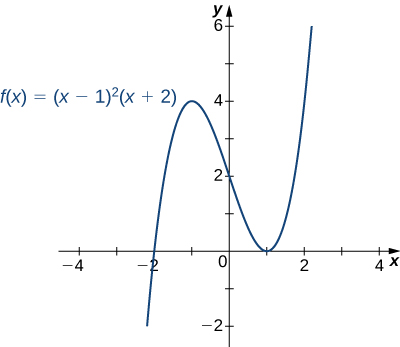
Sketch a graph of [latex]f(x)=(x-1)^2 (x+2)[/latex].
Answer:
Step 1. Since [latex]f[/latex] is a polynomial, the domain is the set of all real numbers.
Step 2. When [latex]x=0, \, f(x)=2[/latex]. Therefore, the [latex]y[/latex]-intercept is [latex](0,2)[/latex]. To find the [latex]x[/latex]-intercepts, we need to solve the equation [latex](x-1)^2 (x+2)=0[/latex], which gives us the [latex]x[/latex]-intercepts [latex](1,0)[/latex] and [latex](-2,0)[/latex]
Step 3. We need to evaluate the end behavior of [latex]f[/latex]. As [latex]x\to \infty[/latex], [latex](x-1)^2 \to \infty [/latex] and [latex](x+2)\to \infty[/latex]. Therefore, [latex]\underset{x\to \infty }{\lim}f(x)=\infty[/latex]. As [latex]x\to −\infty[/latex], [latex](x-1)^2 \to \infty [/latex] and [latex](x+2) \to −\infty[/latex]. Therefore, [latex]\underset{x\to -\infty }{\lim}f(x)=−\infty[/latex]. To get even more information about the end behavior of [latex]f[/latex], we can multiply the factors of [latex]f[/latex]. When doing so, we see that
Since the leading term of [latex]f[/latex] is [latex]x^3[/latex], we conclude that [latex]f[/latex] behaves like [latex]y=x^3[/latex] as [latex]x\to \pm \infty[/latex].
Step 4. Since [latex]f[/latex] is a polynomial function, it does not have any vertical asymptotes.
Step 5. The first derivative of [latex]f[/latex] is
Therefore, [latex]f[/latex] has two critical points: [latex]x=1,-1[/latex]. Divide the interval [latex](−\infty ,\infty)[/latex] into the three smaller intervals: [latex](−\infty ,-1)[/latex], [latex](-1,1)[/latex], and [latex](1,\infty )[/latex]. Then, choose test points [latex]x=-2[/latex], [latex]x=0[/latex], and [latex]x=2[/latex] from these intervals and evaluate the sign of [latex]f^{\prime}(x)[/latex] at each of these test points, as shown in the following table.
| Interval | Test Point | Sign of Derivative [latex]f^{\prime}(x)=3x^2-3=3(x-1)(x+1)[/latex] | Conclusion |
|---|---|---|---|
| [latex](−\infty ,-1)[/latex] | [latex]x=-2[/latex] | [latex](+)(−)(−)=+[/latex] | [latex]f[/latex] is increasing. |
| [latex](-1,1)[/latex] | [latex]x=0[/latex] | [latex](+)(−)(+)=−[/latex] | [latex]f[/latex] is decreasing. |
| [latex](1,\infty )[/latex] | [latex]x=2[/latex] | [latex](+)(+)(+)=+[/latex] | [latex]f[/latex] is increasing. |
From the table, we see that [latex]f[/latex] has a local maximum at [latex]x=-1[/latex] and a local minimum at [latex]x=1[/latex]. Evaluating [latex]f(x)[/latex] at those two points, we find that the local maximum value is [latex]f(-1)=4[/latex] and the local minimum value is [latex]f(1)=0[/latex].
Step 6. The second derivative of [latex]f[/latex] is
The second derivative is zero at [latex]x=0[/latex]. Therefore, to determine the concavity of [latex]f[/latex], divide the interval [latex](−\infty ,\infty)[/latex] into the smaller intervals [latex](−\infty ,0)[/latex] and [latex](0,\infty )[/latex], and choose test points [latex]x=-1[/latex] and [latex]x=1[/latex] to determine the concavity of [latex]f[/latex] on each of these smaller intervals as shown in the following table.
| Interval | Test Point | Sign of [latex]f^{\prime \prime}(x)=6x[/latex] | Conclusion |
|---|---|---|---|
| [latex](−\infty ,0)[/latex] | [latex]x=-1[/latex] | [latex]-[/latex] | [latex]f[/latex] is concave down. |
| [latex](0,\infty )[/latex] | [latex]x=1[/latex] | [latex]+[/latex] | [latex]f[/latex] is concave up. |
We note that the information in the preceding table confirms the fact, found in step 5, that [latex]f[/latex] has a local maximum at [latex]x=-1[/latex] and a local minimum at [latex]x=1[/latex]. In addition, the information found in step 5—namely, [latex]f[/latex] has a local maximum at [latex]x=-1[/latex] and a local minimum at [latex]x=1[/latex], and [latex]f^{\prime}(x)=0[/latex] at those points—combined with the fact that [latex]f^{\prime \prime}[/latex] changes sign only at [latex]x=0[/latex] confirms the results found in step 6 on the concavity of [latex]f[/latex].
Combining this information, we arrive at the graph of [latex]f(x)=(x-1)^2 (x+2)[/latex] shown in the following graph.
Sketch a graph of [latex]f(x)=(x-1)^3 (x+2)[/latex].
Answer: 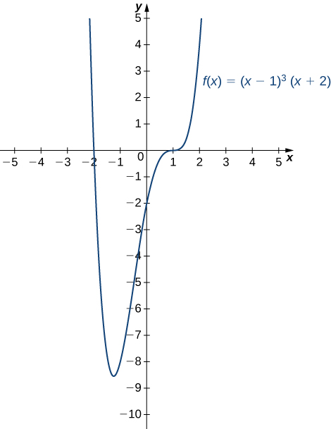
Hint
[latex]f[/latex] is a fourth-degree polynomial.
Sketching a Rational Function
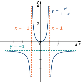
Sketch the graph of [latex]f(x)=\frac{x^2}{1-x^2}[/latex].
Answer:
Step 1. The function [latex]f[/latex] is defined as long as the denominator is not zero. Therefore, the domain is the set of all real numbers [latex]x[/latex] except [latex]x=\pm 1[/latex].
Step 2. Find the intercepts. If [latex]x=0[/latex], then [latex]f(x)=0[/latex], so 0 is an intercept. If [latex]y=0[/latex], then [latex]\frac{x^2}{1-x^2}=0[/latex], which implies [latex]x=0[/latex]. Therefore, [latex](0,0)[/latex] is the only intercept.
Step 3. Evaluate the limits at infinity. Since [latex]f[/latex] is a rational function, divide the numerator and denominator by the highest power in the denominator: [latex]x^2[/latex]. We obtain
Therefore, [latex]f[/latex] has a horizontal asymptote of [latex]y=-1[/latex] as [latex]x\to \infty [/latex] and [latex]x\to −\infty[/latex].
Step 4. To determine whether [latex]f[/latex] has any vertical asymptotes, first check to see whether the denominator has any zeroes. We find the denominator is zero when [latex]x=\pm 1[/latex]. To determine whether the lines [latex]x=1[/latex] or [latex]x=-1[/latex] are vertical asymptotes of [latex]f[/latex], evaluate [latex]\underset{x\to 1}{\lim}f(x)[/latex] and [latex]\underset{x\to −1}{\lim}f(x)[/latex]. By looking at each one-sided limit as [latex]x\to 1[/latex], we see that
In addition, by looking at each one-sided limit as [latex]x\to −1[/latex], we find that
Step 5. Calculate the first derivative:
Critical points occur at points [latex]x[/latex] where [latex]f^{\prime}(x)=0[/latex] or [latex]f^{\prime}(x)[/latex] is undefined. We see that [latex]f^{\prime}(x)=0[/latex] when [latex]x=0[/latex]. The derivative [latex]f^{\prime}[/latex] is not undefined at any point in the domain of [latex]f[/latex]. However, [latex]x=\pm 1[/latex] are not in the domain of [latex]f[/latex]. Therefore, to determine where [latex]f[/latex] is increasing and where [latex]f[/latex] is decreasing, divide the interval [latex](−\infty ,\infty )[/latex] into four smaller intervals: [latex](−\infty ,-1)[/latex], [latex](-1,0)[/latex], [latex](0,1)[/latex], and [latex](1,\infty )[/latex], and choose a test point in each interval to determine the sign of [latex]f^{\prime}(x)[/latex] in each of these intervals. The values [latex]x=-2[/latex], [latex]x=-\frac{1}{2}[/latex], [latex]x=\frac{1}{2}[/latex], and [latex]x=2[/latex] are good choices for test points as shown in the following table.
| Interval | Test Point | Sign of [latex]f^{\prime}(x)=\frac{2x}{(1-x^2)^2}[/latex] | Conclusion |
|---|---|---|---|
| [latex](−\infty ,-1)[/latex] | [latex]x=-2[/latex] | [latex]−/+=−[/latex] | [latex]f[/latex] is decreasing. |
| [latex](-1,0)[/latex] | [latex]x=-1/2[/latex] | [latex]−/+=−[/latex] | [latex]f[/latex] is decreasing. |
| [latex](0,1)[/latex] | [latex]x=1/2[/latex] | [latex]+/+=+[/latex] | [latex]f[/latex] is increasing. |
| [latex](1,\infty )[/latex] | [latex]x=2[/latex] | [latex]+/+=+[/latex] | [latex]f[/latex] is increasing. |
From this analysis, we conclude that [latex]f[/latex] has a local minimum at [latex]x=0[/latex] but no local maximum.
Step 6. Calculate the second derivative:
To determine the intervals where [latex]f[/latex] is concave up and where [latex]f[/latex] is concave down, we first need to find all points [latex]x[/latex] where [latex]f^{\prime \prime}(x)=0[/latex] or [latex]f^{\prime \prime}(x)[/latex] is undefined. Since the numerator [latex]6x^2+2 \ne 0[/latex] for any [latex]x[/latex], [latex]f^{\prime \prime}(x)[/latex] is never zero. Furthermore, [latex]f^{\prime \prime}[/latex] is not undefined for any [latex]x[/latex] in the domain of [latex]f[/latex]. However, as discussed earlier, [latex]x=\pm 1[/latex] are not in the domain of [latex]f[/latex]. Therefore, to determine the concavity of [latex]f[/latex], we divide the interval [latex](−\infty ,\infty )[/latex] into the three smaller intervals [latex](−\infty ,-1)[/latex], [latex](-1,-1)[/latex], and [latex](1,\infty )[/latex], and choose a test point in each of these intervals to evaluate the sign of [latex]f^{\prime \prime}(x)[/latex] in each of these intervals. The values [latex]x=-2[/latex], [latex]x=0[/latex], and [latex]x=2[/latex] are possible test points as shown in the following table.
| Interval | Test Point | Sign of [latex]f^{\prime \prime}(x)=\frac{6x^2+2}{(1-x^2)^3}[/latex] | Conclusion |
|---|---|---|---|
| [latex](−\infty ,-1)[/latex] | [latex]x=-2[/latex] | [latex]+/-=−[/latex] | [latex]f[/latex] is concave down. |
| [latex](-1,-1)[/latex] | [latex]x=0[/latex] | [latex]+/+=+[/latex] | [latex]f[/latex] is concave up. |
| [latex](1,\infty )[/latex] | [latex]x=2[/latex] | [latex]+/-=−[/latex] | [latex]f[/latex] is concave down. |
Combining all this information, we arrive at the graph of [latex]f[/latex] shown below. Note that, although [latex]f[/latex] changes concavity at [latex]x=-1[/latex] and [latex]x=1[/latex], there are no inflection points at either of these places because [latex]f[/latex] is not continuous at [latex]x=-1[/latex] or [latex]x=1[/latex].
Sketch a graph of [latex]f(x)=\frac{3x+5}{8+4x}[/latex].
Answer: 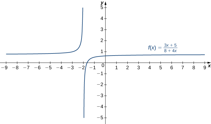
Hint
A line [latex]y=L[/latex] is a horizontal asymptote of [latex]f[/latex] if the limit as [latex]x\to \infty [/latex] or the limit as [latex]x\to −\infty [/latex] of [latex]f(x)[/latex] is [latex]L[/latex]. A line [latex]x=a[/latex] is a vertical asymptote if at least one of the one-sided limits of [latex]f[/latex] as [latex]x\to a[/latex] is [latex]\infty [/latex] or [latex]−\infty[/latex].
Sketching a Rational Function with an Oblique Asymptote
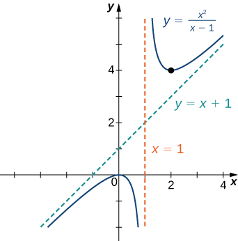
Sketch the graph of [latex]f(x)=\frac{x^2}{x-1}[/latex]
Answer:
Step 1. The domain of [latex]f[/latex] is the set of all real numbers [latex]x[/latex] except [latex]x=1[/latex].
Step 2. Find the intercepts. We can see that when [latex]x=0[/latex], [latex]f(x)=0[/latex], so [latex](0,0)[/latex] is the only intercept.
Step 3. Evaluate the limits at infinity. Since the degree of the numerator is one more than the degree of the denominator, [latex]f[/latex] must have an oblique asymptote. To find the oblique asymptote, use long division of polynomials to write
Since [latex]1/(x-1)\to 0[/latex] as [latex]x\to \pm \infty[/latex], [latex]f(x)[/latex] approaches the line [latex]y=x+1[/latex] as [latex]x\to \pm \infty[/latex]. The line [latex]y=x+1[/latex] is an oblique asymptote for [latex]f[/latex].
Step 4. To check for vertical asymptotes, look at where the denominator is zero. Here the denominator is zero at [latex]x=1[/latex]. Looking at both one-sided limits as [latex]x\to 1[/latex], we find
Therefore, [latex]x=1[/latex] is a vertical asymptote, and we have determined the behavior of [latex]f[/latex] as [latex]x[/latex] approaches 1 from the right and the left.
Step 5. Calculate the first derivative:
We have [latex]f^{\prime}(x)=0[/latex] when [latex]x^2-2x=x(x-2)=0[/latex]. Therefore, [latex]x=0[/latex] and [latex]x=2[/latex] are critical points. Since [latex]f[/latex] is undefined at [latex]x=1[/latex], we need to divide the interval [latex](−\infty ,\infty )[/latex] into the smaller intervals [latex](−\infty ,0)[/latex], [latex](0,1)[/latex], [latex](1,2)[/latex], and [latex](2,\infty )[/latex], and choose a test point from each interval to evaluate the sign of [latex]f^{\prime}(x)[/latex] in each of these smaller intervals. For example, let [latex]x=-1[/latex], [latex]x=\frac{1}{2}[/latex], [latex]x=\frac{3}{2}[/latex], and [latex]x=3[/latex] be the test points as shown in the following table.
| Interval | Test Point | Sign of [latex]f^{\prime}(x)=\frac{x^2-2x}{(x-1)^2}=\frac{x(x-2)}{(x-1)^2}[/latex] | Conclusion |
|---|---|---|---|
| [latex](−\infty ,0)[/latex] | [latex]x=-1[/latex] | [latex](−)(−)/+=+[/latex] | [latex]f[/latex] is increasing. |
| [latex](0,1)[/latex] | [latex]x=1/2[/latex] | [latex](+)(−)/+=−[/latex] | [latex]f[/latex] is decreasing. |
| [latex](1,2)[/latex] | [latex]x=3/2[/latex] | [latex](+)(−)/+=−[/latex] | [latex]f[/latex] is decreasing. |
| [latex](2,\infty )[/latex] | [latex]x=3[/latex] | [latex](+)(+)/+=+[/latex] | [latex]f[/latex] is increasing. |
From this table, we see that [latex]f[/latex] has a local maximum at [latex]x=0[/latex] and a local minimum at [latex]x=2[/latex]. The value of [latex]f[/latex] at the local maximum is [latex]f(0)=0[/latex] and the value of [latex]f[/latex] at the local minimum is [latex]f(2)=4[/latex]. Therefore, [latex](0,0)[/latex] and [latex](2,4)[/latex] are important points on the graph.
Step 6. Calculate the second derivative:
We see that [latex]f^{\prime \prime}(x)[/latex] is never zero or undefined for [latex]x[/latex] in the domain of [latex]f[/latex]. Since [latex]f[/latex] is undefined at [latex]x=1[/latex], to check concavity we just divide the interval [latex](−\infty ,\infty )[/latex] into the two smaller intervals [latex](−\infty ,1)[/latex] and [latex](1,\infty )[/latex], and choose a test point from each interval to evaluate the sign of [latex]f^{\prime \prime}(x)[/latex] in each of these intervals. The values [latex]x=0[/latex] and [latex]x=2[/latex] are possible test points as shown in the following table.
| Interval | Test Point | Sign of [latex]f^{\prime \prime}(x)=\frac{2}{(x-1)^3}[/latex] | Conclusion |
|---|---|---|---|
| [latex](−\infty ,1)[/latex] | [latex]x=0[/latex] | [latex]+/-=−[/latex] | [latex]f[/latex] is concave down. |
| [latex](1,\infty )[/latex] | [latex]x=2[/latex] | [latex]+/+=+[/latex] | [latex]f[/latex] is concave up. |
From the information gathered, we arrive at the following graph for [latex]f.[/latex]
Find the oblique asymptote for [latex]f(x)=\frac{3x^3-2x+1}{2x^2-4}[/latex].
Answer:
[latex]y=\frac{3}{2}x[/latex]
Hint
Use long division of polynomials.
Sketching the Graph of a Function with a Cusp
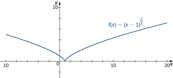
Sketch a graph of [latex]f(x)=(x-1)^{2/3}[/latex].
Answer:
Step 1. Since the cube-root function is defined for all real numbers [latex]x[/latex] and [latex](x-1)^{2/3}=(\sqrt[3]{x-1})^2[/latex], the domain of [latex]f[/latex] is all real numbers.
Step 2: To find the [latex]y[/latex]-intercept, evaluate [latex]f(0)[/latex]. Since [latex]f(0)=1[/latex], the [latex]y[/latex]-intercept is [latex](0,1)[/latex]. To find the [latex]x[/latex]-intercept, solve [latex](x-1)^{2/3}=0[/latex]. The solution of this equation is [latex]x=1[/latex], so the [latex]x[/latex]-intercept is [latex](1,0)[/latex].
Step 3: Since [latex]\underset{x\to \pm \infty }{\lim}(x-1)^{2/3}=\infty [/latex], the function continues to grow without bound as [latex]x\to \infty [/latex] and [latex]x\to −\infty[/latex].
Step 4: The function has no vertical asymptotes.
Step 5: To determine where [latex]f[/latex] is increasing or decreasing, calculate [latex]f^{\prime}[/latex]. We find
This function is not zero anywhere, but it is undefined when [latex]x=1[/latex]. Therefore, the only critical point is [latex]x=1[/latex]. Divide the interval [latex](−\infty ,\infty )[/latex] into the smaller intervals [latex](−\infty ,1)[/latex] and [latex](1,\infty )[/latex], and choose test points in each of these intervals to determine the sign of [latex]f^{\prime}(x)[/latex] in each of these smaller intervals. Let [latex]x=0[/latex] and [latex]x=2[/latex] be the test points as shown in the following table.
| Interval | Test Point | Sign of [latex]f^{\prime}(x)=\frac{2}{3(x-1)^{1/3}}[/latex] | Conclusion |
|---|---|---|---|
| [latex](−\infty ,1)[/latex] | [latex]x=0[/latex] | [latex]+/-=−[/latex] | [latex]f[/latex] is decreasing. |
| [latex](1,\infty )[/latex] | [latex]x=2[/latex] | [latex]+/+=+[/latex] | [latex]f[/latex] is increasing. |
We conclude that [latex]f[/latex] has a local minimum at [latex]x=1[/latex]. Evaluating [latex]f[/latex] at [latex]x=1[/latex], we find that the value of [latex]f[/latex] at the local minimum is zero. Note that [latex]f^{\prime}(1)[/latex] is undefined, so to determine the behavior of the function at this critical point, we need to examine [latex]\underset{x\to 1}{\lim}f^{\prime}(x)[/latex]. Looking at the one-sided limits, we have
Therefore, [latex]f[/latex] has a cusp at [latex]x=1[/latex].
Step 6: To determine concavity, we calculate the second derivative of [latex]f[/latex]:
We find that [latex]f^{\prime \prime}(x)[/latex] is defined for all [latex]x[/latex], but is undefined when [latex]x=1[/latex]. Therefore, divide the interval [latex](−\infty ,\infty )[/latex] into the smaller intervals [latex](−\infty ,1)[/latex] and [latex](1,\infty )[/latex], and choose test points to evaluate the sign of [latex]f^{\prime \prime}(x)[/latex] in each of these intervals. As we did earlier, let [latex]x=0[/latex] and [latex]x=2[/latex] be test points as shown in the following table.
| Interval | Test Point | Sign of [latex]f^{\prime \prime}(x)=\frac{-2}{9(x-1)^{4/3}}[/latex] | Conclusion |
|---|---|---|---|
| [latex](−\infty ,1)[/latex] | [latex]x=0[/latex] | [latex]−/+=−[/latex] | [latex]f[/latex] is concave down. |
| [latex](1,\infty )[/latex] | [latex]x=2[/latex] | [latex]−/+=−[/latex] | [latex]f[/latex] is concave down. |
From this table, we conclude that [latex]f[/latex] is concave down everywhere. Combining all of this information, we arrive at the following graph for [latex]f[/latex].
Consider the function [latex]f(x)=5-x^{2/3}[/latex]. Determine the point on the graph where a cusp is located. Determine the end behavior of [latex]f[/latex].
Answer:
The function [latex]f[/latex] has a cusp at [latex](0,5)[/latex]: [latex]\underset{x\to 0^-}{\lim}f^{\prime}(x)=\infty[/latex], [latex]\underset{x\to 0^+}{\lim}f^{\prime}(x)=−\infty[/latex]. For end behavior, [latex]\underset{x\to \pm \infty }{\lim}f(x)=−\infty[/latex].
Hint
A function [latex]f[/latex] has a cusp at a point [latex]a[/latex] if [latex]f(a)[/latex] exists, [latex]f^{\prime}(a)[/latex] is undefined, one of the one-sided limits as [latex]x\to a[/latex] of [latex]f^{\prime}(x)[/latex] is [latex]+\infty[/latex], and the other one-sided limit is [latex]−\infty[/latex].
Key Concepts
- If [latex]f^{\prime \prime}(x)>0[/latex] over an interval [latex]I[/latex], then [latex]f[/latex] is concave up over [latex]I[/latex].
- If [latex]f^{\prime \prime}(x)<0[/latex] over an interval [latex]I[/latex], then [latex]f[/latex] is concave down over [latex]I[/latex].
- If [latex]f^{\prime}(c)=0[/latex] and [latex]f^{\prime \prime}(c)>0[/latex], then [latex]f[/latex] has a local minimum at [latex]c[/latex].
- If [latex]f^{\prime}(c)=0[/latex] and [latex]f^{\prime \prime}(c)<0[/latex], then [latex]f[/latex] has a local maximum at [latex]c[/latex].
- If [latex]f^{\prime}(c)=0[/latex] and [latex]f^{\prime \prime}(c)=0[/latex], then evaluate [latex]f^{\prime}(x)[/latex] at a test point [latex]x[/latex] to the left of [latex]c[/latex] and a test point [latex]x[/latex] to the right of [latex]c[/latex], to determine whether [latex]f[/latex] has a local extremum at [latex]c[/latex].
- For a polynomial function [latex]p(x)=a_n x^n + a_{n-1} x^{n-1} + \cdots + a_1 x + a_0[/latex], where [latex]a_n \ne 0[/latex], the end behavior is determined by the leading term [latex]a_n x^n[/latex]. If [latex]n\ne 0[/latex], [latex]p(x)[/latex] approaches [latex]\infty [/latex] or [latex]−\infty [/latex] at each end.
- For a rational function [latex]f(x)=\frac{p(x)}{q(x)}[/latex], the end behavior is determined by the relationship between the degree of [latex]p[/latex] and the degree of [latex]q[/latex]. If the degree of [latex]p[/latex] is less than the degree of [latex]q[/latex], the line [latex]y=0[/latex] is a horizontal asymptote for [latex]f[/latex]. If the degree of [latex]p[/latex] is equal to the degree of [latex]q[/latex], then the line [latex]y=\frac{a_n}{b_n}[/latex] is a horizontal asymptote, where [latex]a_n[/latex] and [latex]b_n[/latex] are the leading coefficients of [latex]p[/latex] and [latex]q[/latex], respectively. If the degree of [latex]p[/latex] is greater than the degree of [latex]q[/latex], then [latex]f[/latex] approaches [latex]\infty [/latex] or [latex]−\infty [/latex] at each end.
2. For the function [latex]y=x^3[/latex], is [latex]x=0[/latex] both an inflection point and a local maximum/minimum?
Answer:
It is not a local maximum/minimum because [latex]f^{\prime}[/latex] does not change sign
3. For the function [latex]y=x^3[/latex], is [latex]x=0[/latex] an inflection point?
4. Is it possible for a point [latex]c[/latex] to be both an inflection point and a local extrema of a twice differentiable function?
Answer:
No
5. Why do you need continuity for the first derivative test? Come up with an example.
6. Explain whether a concave-down function has to cross [latex]y=0[/latex] for some value of [latex]x[/latex].
Answer:
False; for example, [latex]y=\sqrt{x}[/latex].
7. Explain whether a polynomial of degree 2 can have an inflection point.
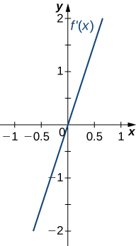
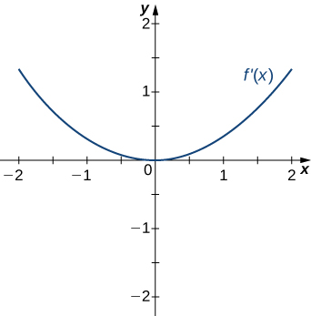
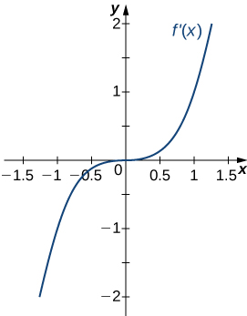
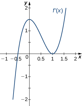
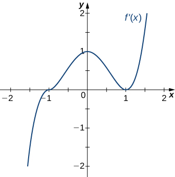
For the following exercises, analyze the graphs of [latex]f^{\prime}[/latex], then list all inflection points and intervals [latex]f[/latex] that are concave up and concave down.
Answer:
Concave up on all [latex]x[/latex], no inflection points
Answer: Concave up on all [latex]x[/latex], no inflection points
Answer:
Concave up for [latex]x<0[/latex] and [latex]x>1[/latex], concave down for [latex]0<x<1[/latex], inflection points at [latex]x=0[/latex] and [latex]x=1[/latex]
For the following exercises, draw a graph that satisfies the given specifications for the domain [latex]x=[-3,3][/latex]. The function does not have to be continuous or differentiable.
23. [latex]f(x)>0, \, f^{\prime}(x)>0[/latex] over [latex]x>1, \, -3<x<0, \, f^{\prime}(x)=0[/latex] over [latex]0<x<1[/latex]
24. [latex]f^{\prime}(x)>0[/latex] over [latex]x>2, \, -3<x<-1, \, f^{\prime}(x)<0[/latex] over [latex]-1<x<2, \, f^{\prime \prime}(x)<0[/latex] for all [latex]x[/latex]
Answer:
Answers will vary
25. [latex]f^{\prime \prime}(x)<0[/latex] over [latex]-1<x<1, \, f^{\prime \prime}(x)>0, \, -3<x<-1, \, 1<x<3[/latex], local maximum at [latex]x=0[/latex], local minima at [latex]x=\pm 2[/latex]
26. There is a local maximum at [latex]x=2[/latex], local minimum at [latex]x=1[/latex], and the graph is neither concave up nor concave down.
Answer:
Answers will vary
27. There are local maxima at [latex]x=\pm 1[/latex], the function is concave up for all [latex]x[/latex], and the function remains positive for all [latex]x[/latex].
For the following exercise, determine a. intervals where [latex]f[/latex] is concave up or concave down, and b. the inflection points of [latex]f[/latex].
30. [latex]f(x)=x^3-4x^2+x+2[/latex]
Answer:
a. Concave up for [latex]x>\frac{4}{3}[/latex], concave down for [latex]x<\frac{4}{3}[/latex] b. Inflection point at [latex]x=\frac{4}{3}[/latex]
For the following exercises, determine
- intervals where [latex]f[/latex] is increasing or decreasing,
- local minima and maxima of [latex]f[/latex],
- intervals where [latex]f[/latex] is concave up and concave down, and
- the inflection points of [latex]f[/latex].
31. [latex]f(x)=x^2-6x[/latex]
32. [latex]f(x)=x^3-6x^2[/latex]
Answer:
a. Increasing over [latex]x<0[/latex] and [latex]x>4[/latex], decreasing over [latex]0<x<4[/latex] b. Maximum at [latex]x=0[/latex], minimum at [latex]x=4[/latex] c. Concave up for [latex]x>2[/latex], concave down for [latex]x<2[/latex] d. Infection point at [latex]x=2[/latex]
33. [latex]f(x)=x^4-6x^3[/latex]
34. [latex]f(x)=x^{11}-6x^{10}[/latex]
Answer:
a. Increasing over [latex]x<0[/latex] and [latex]x>\frac{60}{11}[/latex], decreasing over [latex]0<x<\frac{60}{11}[/latex] b. Minimum at [latex]x=\frac{60}{11}[/latex] c. Concave down for [latex]x<\frac{54}{11}[/latex], concave up for [latex]x>\frac{54}{11}[/latex] d. Inflection point at [latex]x=\frac{54}{11}[/latex]
35. [latex]f(x)=x+x^2-x^3[/latex]
36. [latex]f(x)=x^2+x+1[/latex]
Answer:
a. Increasing over [latex]x>-\frac{1}{2}[/latex], decreasing over [latex]x<-\frac{1}{2}[/latex] b. Minimum at [latex]x=-\frac{1}{2}[/latex] c. Concave up for all [latex]x[/latex] d. No inflection points
37. [latex]f(x)=x^3+x^4[/latex]
For the following exercises, determine
- intervals where [latex]f[/latex] is increasing or decreasing,
- local minima and maxima of [latex]f[/latex],
- intervals where [latex]f[/latex] is concave up and concave down, and
- the inflection points of [latex]f[/latex]. Sketch the curve, then use a calculator to compare your answer. If you cannot determine the exact answer analytically, use a calculator.
38. [T] [latex]f(x)= \sin (\pi x)- \cos (\pi x)[/latex] over [latex]x=[-1,1][/latex]
Answer:
a. Increases over [latex]-\frac{1}{4}<x<\frac{3}{4}[/latex], decreases over [latex]x>\frac{3}{4}[/latex] and [latex]x<-\frac{1}{4}[/latex] b. Minimum at [latex]x=-\frac{1}{4}[/latex], maximum at [latex]x=\frac{3}{4}[/latex] c. Concave up for [latex]-\frac{3}{4}<x<\frac{1}{4}[/latex], concave down for [latex]x<-\frac{3}{4}[/latex] and [latex]x>\frac{1}{4}[/latex] d. Inflection points at [latex]x=-\frac{3}{4}, \, x=\frac{1}{4}[/latex]
39. [T] [latex]f(x)=x + \sin (2x)[/latex] over [latex]x=[-\frac{\pi }{2},\frac{\pi }{2}][/latex]
40. [T] [latex]f(x)= \sin x+ \tan x[/latex] over [latex](-\frac{\pi }{2},\frac{\pi }{2})[/latex]
Answer:
a. Increasing for all [latex]x[/latex] b. No local minimum or maximum c. Concave up for [latex]x>0[/latex], concave down for [latex]x<0[/latex] d. Inflection point at [latex]x=0[/latex]
41. [T] [latex]f(x)=(x-2)^2 (x-4)^2[/latex]
42. [T] [latex]f(x)=\frac{1}{1-x}, \, x \ne 1[/latex]
Answer:
a. Increasing for all [latex]x[/latex] where defined b. No local minima or maxima c. Concave up for [latex]x<1[/latex], concave down for [latex]x>1[/latex] d. No inflection points in domain
43. [T] [latex]f(x)=\frac{\sin x}{x}[/latex] over [latex]x=[-2\pi ,0) \cup (0,2\pi][/latex]
44. [latex]f(x)= \sin x e^x[/latex] over [latex]x=[−\pi ,\pi][/latex]
Answer:
a. Increasing over [latex]-\frac{\pi }{4}<x<\frac{3\pi }{4}[/latex], decreasing over [latex]x>\frac{3\pi }{4}, \, x<-\frac{\pi }{4}[/latex] b. Minimum at [latex]x=-\frac{\pi }{4}[/latex], maximum at [latex]x=\frac{3\pi }{4}[/latex] c. Concave up for [latex]-\frac{\pi }{2}<x<\frac{\pi }{2}[/latex], concave down for [latex]x<-\frac{\pi }{2}, \, x>\frac{\pi }{2}[/latex] d. Infection points at [latex]x=\pm \frac{\pi }{2}[/latex]
45. [latex]f(x)=\ln x \sqrt{x}, \, x>0[/latex]
46. [latex]f(x)=\frac{1}{4}\sqrt{x}+\frac{1}{x}, \, x>0[/latex]
Answer:
a. Increasing over [latex]x>4[/latex], decreasing over [latex]0<x<4[/latex] b. Minimum at [latex]x=4[/latex] c. Concave up for [latex]0<x<8\sqrt[3]{2}[/latex], concave down for [latex]x>8\sqrt[3]{2}[/latex] d. Inflection point at [latex]x=8\sqrt[3]{2}[/latex]
47. [latex]f(x)=\frac{e^x}{x}, \, x\ne 0[/latex]
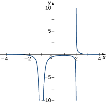
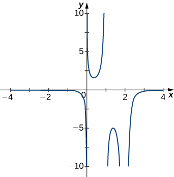
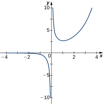
For the following exercises, examine the graphs. Identify where the vertical asymptotes are located.
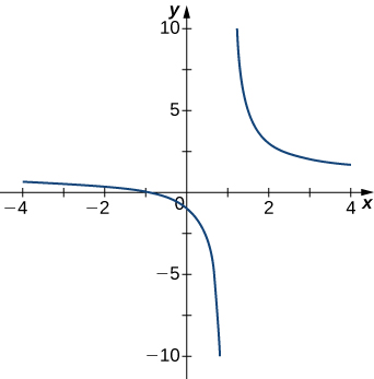
Answer:
[latex]x=1[/latex]
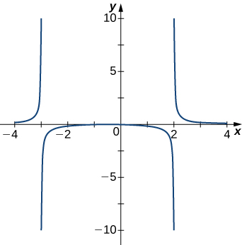
Answer:
[latex]x=-1, \, x=2[/latex]
Answer:
[latex]x=0[/latex]
For the following functions [latex]f(x)[/latex], determine whether there is an asymptote at [latex]x=a[/latex]. Justify your answer without graphing on a calculator.
6. [latex]f(x)=\frac{x+1}{x^2+5x+4}, \, a=-1[/latex]
7. [latex]f(x)=\frac{x}{x-2}, \, a=2[/latex]
Answer:
Yes, there is a vertical asymptote
8. [latex]f(x)=(x+2)^{3/2}, \, a=-2[/latex]
9. [latex]f(x)=(x-1)^{-1/3}, \, a=1[/latex]
Answer:
Yes, there is a vertical asymptote
10. [latex]f(x)=1+x^{-2/5}, \, a=1[/latex]
For the following exercises, construct a function [latex]f(x)[/latex] that has the given asymptotes.
11. [latex]x=1[/latex] and [latex]y=2[/latex]
Answer:
Answers will vary, for example: [latex]y=\frac{2x}{x-1}[/latex]
12. [latex]x=1[/latex] and [latex]y=0[/latex]
13. [latex]y=4[/latex] and [latex]x=-1[/latex]
Answer:
Answers will vary, for example: [latex]y=\frac{4x}{x+1}[/latex]
14. [latex]x=0[/latex]
For the following exercises, graph the function on a graphing calculator on the window [latex]x=[-5,5][/latex] and estimate the horizontal asymptote or limit. Then, calculate the actual horizontal asymptote or limit.
15. [T] [latex]f(x)=\frac{1}{x+10}[/latex]
Answer:
[latex]y=0[/latex]
16. [T] [latex]f(x)=\frac{x+1}{x^2+7x+6}[/latex]
17. [T] [latex]\underset{x\to −\infty }{\lim} x^2+10x+25[/latex]
Answer:
[latex]\infty [/latex]
18. [T] [latex]\underset{x\to −\infty }{\lim}\frac{x+2}{x^2+7x+6}[/latex]
19. [T] [latex]\underset{x\to \infty }{\lim}\frac{3x+2}{x+5}[/latex]
Answer:
[latex]y=3[/latex]
For the following exercises, draw a graph of the functions without using a calculator. Be sure to notice all important features of the graph: local maxima and minima, inflection points, and asymptotic behavior.
20. [latex]y=3x^2+2x+4[/latex]
21. [latex]y=x^3-3x^2+4[/latex]
Answer: 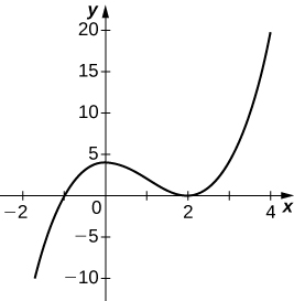
22. [latex]y=\frac{2x+1}{x^2+6x+5}[/latex]
23. [latex]y=\frac{x^3+4x^2+3x}{3x+9}[/latex]
Answer: 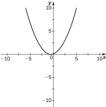
24. [latex]y=\frac{x^2+x-2}{x^2-3x-4}[/latex]
25. [latex]y=\sqrt{x^2-5x+4}[/latex]
Answer: 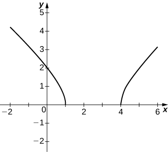
26. [latex]y=2x\sqrt{16-x^2}[/latex]
27. [latex]y=\frac{ \cos x}{x}[/latex], on [latex]x=[-2\pi ,2\pi][/latex]
Answer: 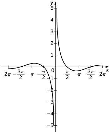
28. [latex]y=e^x-x^3[/latex]
29. [latex]y=x \tan x, \, x=[−\pi ,\pi][/latex]
Answer: 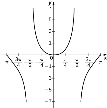
30. [latex]y=x \ln (x), \, x>0[/latex]
31. [latex]y=x^2 \sin (x), \, x=[-2\pi ,2\pi][/latex]
Answer: 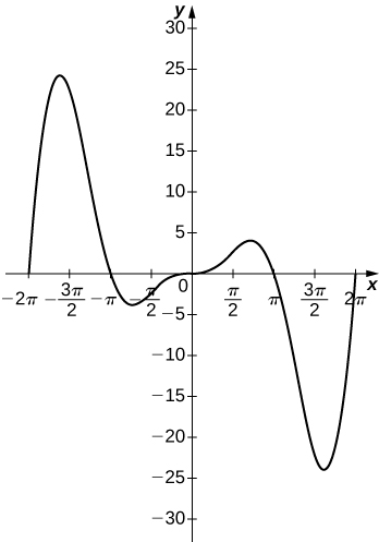
32. For [latex]f(x)=\frac{P(x)}{Q(x)}[/latex] to have an asymptote at [latex]y=2[/latex] then the polynomials [latex]P(x)[/latex] and [latex]Q(x)[/latex] must have what relation?
33. For [latex]f(x)=\frac{P(x)}{Q(x)}[/latex] to have an asymptote at [latex]x=0[/latex], then the polynomials [latex]P(x)[/latex] and [latex]Q(x)[/latex] must have what relation?
Answer:
[latex]Q(x)[/latex] must have have [latex]x^{k+1}[/latex] as a factor, where [latex]P(x)[/latex] has [latex]x^k[/latex] as a factor.
34. If [latex]f^{\prime}(x)[/latex] has asymptotes at [latex]y=3[/latex] and [latex]x=1[/latex], then [latex]f(x)[/latex] has what asymptotes?
35. Both [latex]f(x)=\frac{1}{x-1}[/latex] and [latex]g(x)=\frac{1}{(x-1)^2}[/latex] have asymptotes at [latex]x=1[/latex] and [latex]y=0[/latex]. What is the most obvious difference between these two functions?
Answer:
[latex]\underset{x\to 1^-}{\lim} f(x)[/latex] and [latex]\underset{x\to 1^-}{\lim} g(x)[/latex]
36. True or false: Every ratio of polynomials has vertical asymptotes.
Glossary
- end behavior
- the behavior of a function as [latex]x\to \infty [/latex] and [latex]x\to −\infty [/latex]
- horizontal asymptote
- if [latex]\underset{x\to \infty }{\lim}f(x)=L[/latex] or [latex]\underset{x\to −\infty }{\lim}f(x)=L[/latex], then [latex]y=L[/latex] is a horizontal asymptote of [latex]f[/latex]
- infinite limit at infinity
- a function that becomes arbitrarily large as [latex]x[/latex] becomes large
- limit at infinity
- the limiting value, if it exists, of a function as [latex]x\to \infty [/latex] or [latex]x\to −\infty [/latex]
- oblique asymptote
- the line [latex]y=mx+b[/latex] if [latex]f(x)[/latex] approaches it as [latex]x\to \infty [/latex] or [latex]x\to −\infty [/latex]
Key Concepts
- If [latex]c[/latex] is a critical point of [latex]f[/latex] and [latex]f^{\prime}(x)>0[/latex] for [latex]x<c[/latex] and [latex]f^{\prime}(x)<0[/latex] for [latex]x>c[/latex], then [latex]f[/latex] has a local maximum at [latex]c[/latex].
- If [latex]c[/latex] is a critical point of [latex]f[/latex] and [latex]f^{\prime}(x)<0[/latex] for [latex]x<c[/latex] and [latex]f^{\prime}(x)>0[/latex] for [latex]x>c[/latex], then [latex]f[/latex] has a local minimum at [latex]c[/latex].
- If [latex]f^{\prime \prime}(x)>0[/latex] over an interval [latex]I[/latex], then [latex]f[/latex] is concave up over [latex]I[/latex].
- If [latex]f^{\prime \prime}(x)<0[/latex] over an interval [latex]I[/latex], then [latex]f[/latex] is concave down over [latex]I[/latex].
- If [latex]f^{\prime}(c)=0[/latex] and [latex]f^{\prime \prime}(c)>0[/latex], then [latex]f[/latex] has a local minimum at [latex]c[/latex].
- If [latex]f^{\prime}(c)=0[/latex] and [latex]f^{\prime \prime}(c)<0[/latex], then [latex]f[/latex] has a local maximum at [latex]c[/latex].
- If [latex]f^{\prime}(c)=0[/latex] and [latex]f^{\prime \prime}(c)=0[/latex], then evaluate [latex]f^{\prime}(x)[/latex] at a test point [latex]x[/latex] to the left of [latex]c[/latex] and a test point [latex]x[/latex] to the right of [latex]c[/latex], to determine whether [latex]f[/latex] has a local extremum at [latex]c[/latex].

Hint
Find where [latex]f^{\prime \prime}(x)=0[/latex].