G1.07: Section 4
Optional Section 4: Adding formatting to the spreadsheet used to explore parameter values. When you are just creating a spreadsheet to use for a few minutes, it is easy to remember what you put where and what it meant. But it is also convenient to save some worksheets and use them again later. When you do that, it is good to add some features that make it easier to remember what is where. In this course, we will add several features to such spreadsheets.- We will make the cells in which we change numerical values green, so that it is easy to see at a glance what to change.
- We will make the cells that are computed from those values we change yellow, so that it is easy to look at what numbers changed as a result of what we entered.
- We will add a line that shows the formula with the numerical values we are using.
Methods
Color:
To make cells a given color, choose the cells (highlight them) and, from the menu, choose Format > Cells and then choose the “Patterns” tab. From there, choose the color you want. In this course, we will use green for input and yellow for computed values. (We will also use blue for cells where there is a “check.” That has not yet been illustrated in the examples.)Formula:
To show the formula in the spreadsheet for Example 16 above in cell G1, use Excel’s CONCATENATE function in the following way. In G1 enter =CONCATENATE("y=",G3," x + ",G2)
| A | B | C | D | E | F | G | H | |
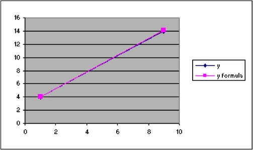
| 1 | x | y | y formula | y=2.8 x + 1.25 | ||||
| 2 | 1 | 4 | 4.05 | 2.8 | intercept | |||
| 3 | 9 | 14 | 14.05 | 1.25 | slope | |||
| 4 | ||||||||
| 5 | ||||||||
| 6 | ||||||||
| 7 | ||||||||
| 8 | ||||||||
| 9 | ||||||||
| 10 | ||||||||
| 11 | ||||||||
| 12 | ||||||||
| 13 | ||||||||
| 14 | ||||||||
| 15 | ||||||||
| 16 | ||||||||
Licenses & Attributions
CC licensed content, Shared previously
- Mathematics for Modeling. Authored by: Mary Parker and Hunter Ellinger. License: CC BY: Attribution.
