Differential Equations
Solving Differential Equations
Differential equations are solved by finding the function for which the equation holds true.
Learning Objectives
Calculate the order and degree of a differential equation.
Key Takeaways
Key Points
- The order of a differential equation is determined by the highest-order derivative; the degree is determined by the highest power on a variable.
- The higher the order of the differential equation, the more arbitrary constants need to be added to the general solution. A first-order equation will have one, a second-order two, and so on.
- A particular solution can be found by assigning values to the arbitrary constants to match any given constraints.
Key Terms
- function: a relation in which each element of the domain is associated with exactly one element of the co-domain
- derivative: a measure of how a function changes as its input changes
A differential equation is a mathematical equation for an unknown function of one or several variables that relates the values of the function itself to its derivatives of various orders. Differential equations play a prominent role in engineering, physics, economics, and other disciplines.
Differential equations take a form similar to:
f(x)+f′(x)=0
where
f′ is "f-prime," the derivative of
f. As you can see, such an equation relates a function
f(x) to its derivative. Solving the differential equation means solving for the function
f(x).
The "order" of a differential equation depends on the derivative of the highest order in the equation. The "degree" of a differential equation, similarly, is determined by the highest exponent on any variables involved. For example, the differential equation shown in is of second-order, third-degree, and the one above is of first-order, first-degree.
Solving a Differential Equation: A Simple Example
Take the following differential equation:
f(x)+f′(x)=0
This equation states that
f(x) is equal to the negative of its derivative. You may recall that one function that satisfies this property is
f(x) =
e−x. The derivative of
f(x)
equals -
e−x i.e. -
f(x) so this function solves the differential equation.
A complete solution contains the same number of arbitrary constants as the order of the original equation. (This is because, in order to solve a differential equation of the
nth order, you will integrate
n times, each time adding a new arbitrary constant.) Since our example above is a first-order equation, it will have just one arbitrary constant in the complete solution. Therefore, the general solution is
f(x)=Ce−x, where
C stands for an arbitrary constant. You can see that the differential equation still holds true with this constant. For a specific solution, replace the constants in the general solution with actual numeric values.
Models Using Differential Equations
Differential equations can be used to model a variety of physical systems.
Learning Objectives
Give examples of systems that can be modeled with differential equations
Key Takeaways
Key Points
- Many systems can be well understood through differential equations.
- Mathematical models of differential equations can be used to solve problems and generate models.
- An example of such a model is the differential equation governing radioactive decay.
Key Terms
- differential equation: an equation involving the derivatives of a function
- decay: To change by undergoing fission, by emitting radiation, or by capturing or losing one or more electrons.
Differential equations are very important in the mathematical modeling of physical systems.
Many fundamental laws of physics and chemistry can be formulated as differential equations. In biology and economics, differential equations are used to model the behavior of complex systems. The mathematical theory of differential equations first developed together with the sciences where the equations had originated and where the results found application. However, diverse problems, sometimes originating in quite distinct scientific fields, may give rise to identical differential equations. Whenever this happens, mathematical theory behind the equations can be viewed as a unifying principle behind diverse phenomena. As an example, consider propagation of light and sound in the atmosphere, and of waves on the surface of a pond. All of them may be described by the same second-order partial-differential equation, the wave equation, which allows us to think of light and sound as forms of waves, much like familiar waves in the water. Conduction of heat is governed by another second-order partial differential equation, the heat equation.
A good example of a physical system modeled with differential equations is radioactive decay in physics.
Over time, radioactive elements decay. The half-life,
t1/2, is the time taken for the activity of a given amount of a radioactive substance to decay to half of its initial value. The mean lifetime,
τ ("tau"), is the average lifetime of a radioactive particle before decay. The decay constant,
λ ("lambda"), is the inverse of the mean lifetime.
We can combine these quantities in a differential equation to determine the activity of the substance. For a number of radioactive particles
N, the activity
A, or number of decays per time is given by:
A=−dtdN=λN
a first-order differential equation.
Direction Fields and Euler's Method
Direction fields and Euler's method are ways of visualizing and approximating the solutions to differential equations.
Learning Objectives
Describe application of direction fields and Euler's method to approximate the solutions to differential equations
Key Takeaways
Key Points
- Direction fields, or slope fields, are graphs where each point (x,y) has a slope.
- Euler's method is a way of approximating solutions to differential equations by assuming that the slope at a point is the same as the slope between that point and the next point.
- Euler's method gives approximate solutions to differential equations, and the smaller the distance between the chosen points, the more accurate the result.
Key Terms
- tangent: a straight line touching a curve at a single point without crossing it there
- differential equation: an equation involving the derivatives of a function
- normalize: (in mathematics) to divide a vector by its magnitude to produce a unit vector
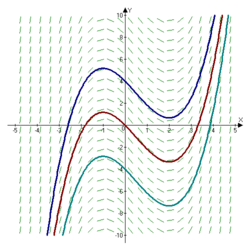
Direction Fields
Direction fields, also known as slope fields, are graphical representations of the solution to a first order differential equation. They can be achieved without solving the differential equation analytically, and serve as a useful way to visualize the solutions.
The slope field is traditionally defined for differential equations of the following form:
y′=f(x)
It can be viewed as a creative way to plot a real-valued function of two real variables as a planar picture.
Specifically, for a given pair, a vector with the components is drawn at the point
(x,y) on the
xy-plane. Sometimes, the vector is normalized to make the plot more pleasing to the human eye. A set of pairs
(x,y) making a rectangular grid is typically used for the drawing. An isocline (a series of lines with the same slope) is often used to supplement the slope field. In an equation of the form, the isocline is a line in the
xy-plane obtained by setting
f(x,y) equal to a constant.
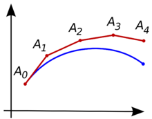
Euler's Method
Consider the problem of calculating the shape of an unknown curve which starts at a given point and satisfies a given differential equation. Here, a differential equation can be thought of as a formula by which the slope of the tangent line to the curve can be computed at any point on the curve, once the position of that point has been calculated.The idea is that while the curve is initially unknown, its starting point, which we denote by
A0, is known (see ). Then, from the differential equation, the slope to the curve at
A0 can be computed, and thus, the tangent line.
Take a small step along that tangent line up to a point,
A1. Along this small step, the slope does not change too much
A1 will be close to the curve. If we pretend that
A1 is still on the curve, the same reasoning we used for the above point,
A0, can be applied. After several steps, a polygonal curve is computed. In general, this curve does not diverge too far from the original unknown curve, and the error between the two curves can be made small if the step size is small enough and the interval of computation is finite.
Separable Equations
Separable differential equations are equations wherein the variables can be separated.
Learning Objectives
Identify steps necessary to solve separable equations
Key Takeaways
Key Points
- Separable equations are of the form M(y)dxdy=N(x).
- Separable equations are among the easiest differential equations to solve.
- To solve, collect all terms that contain the same variables to one side and integrate through.
Key Terms
- fraction: a ratio of two numbers, the numerator and the denominator; usually written one above the other and separated by a horizontal bar
- differential equation: an equation involving the derivatives of a function
- derivative: a measure of how a function changes as its input changes
Non-linear differential equations come in many forms. One of these forms is separable equations. A differential equation that is separable will have several properties which can be exploited to find a solution.
A separable equation is a differential equation of the following form:
N(y)dxdy=M(x)
The original equation is separable if this differential equation can be expressed as:
f(x)dx+g(y)dy=0
where
f(x) is in terms of only
x and
g(y) is in terms of only
y. This is the easiest variety of differential equation to solve. Integrating such an equation yields:
∫f(x)dx+∫g(y)dy=c
where
c is the standard arbitrary constant.
To separate the equations means to move all the
x terms and
ys terms to the opposite sides of the equation.
A general approach to solving separable equations is as follows:
- Multiply and divide to get rid of any fractions.
- Combine any terms involving the same differential into one term.
- Integrate each component on its own, and don't forget to add constants to equations after integrating. This ensures that the solution is of the general form.
- Finally, simplify the expression (i.e., combine all possible terms, rewrite any logarithmic terms in exponent form, and express any arbitrary constants in the most simple terms possible).
After simplifying you will have the general form of the equation. A particular solution to the equation will depend on the choice of the arbitrary constants you obtained when integrating.
For example, consider the time-independent Schrödinger equation:
(−▽2+V(x))⋅ψ(x)=Eψ(x)
If the function
V(x) in three dimensions is of the form
V(x1,x2,x3)=V1(x1)+V2(x2)+V3(x3)
then it turns out that the problem can be separated into three one-dimensional ordinary differential equations for functions:
ψ1(x1),
ψ2(x2),
ψ3(x3).
The final solution can be written as follows:
ψ(x)=ψ1(x1)⋅ψ2(x2)⋅ψ3(x3)
Logistic Equations and Population Grown
A logistic equation is a differential equation which can be used to model population growth.
Learning Objectives
Describe shape of the logistic function and its use for modeling population growth
Key Takeaways
Key Points
- The logistic function initially grows exponentially before slowing down as it reaches a ceiling.
- This behavior makes it a good model for population growth, since populations initially grow rapidly but tend to slow down due to eventual lack of resources.
- Varying the parameters in the equation can simulate various environmental factors which impact population growth.
Key Terms
- derivative: a measure of how a function changes as its input changes
- boundary condition: the set of conditions specified for behavior of the solution to a set of differential equations at the boundary of its domain
- non-linear differential equation: nonlinear partial differential equation is partial differential equation with nonlinear terms
The logistic function is the solution of the following simple first-order non- linear differential equation:
dtdP(t)=P(t)(1−P(t))
with boundary condition
P(0)=21.
The derivative is
0 at
P=0 or
P=1, and the derivative is positive for
0≤P≤1 and negative for
1<P or
P<0 (though negative populations do not generally accord with a physical model). This yields an unstable equilibrium at
0 and a stable equilibrium at
1, and thus for
0<P<1,
P grows to
1. One may readily find the (symbolic) solution to be as follows:
P(t)=et+ecet
Choosing the constant of integration
ec=1 gives the other well-known form of the definition of the logistic curve:
P(t)=et+1et
More quantitatively, as can be seen from the analytical solution, the logistic curve shows early exponential growth for negative
t, which slows to linear growth of slope
41 near
t=0, then approaches
y=1 with an exponentially decaying gap.
The logistic equation is commonly applied as a model of population growth, where the rate of reproduction is proportional to both the existing population and the amount of available resources, all else being equal. The equation describes the self-limiting growth of a biological population.
Letting
P represent population size (
N is often used instead in ecology) and
t represent time, this model is formalized by the following differential equation:
dtdP=rP(1−KP)
where the constant
r defines the growth rate and
K is the carrying capacity. In the equation, the early, unimpeded growth rate is modeled by the first term
rP. The value of the rate
r represents the proportional increase of the population
P in one unit of time. Later, as the population grows, the second term, which multiplied out is
K−rP2, becomes larger than the first as some members of the population
P interfere with each other by competing for some critical resource, such as food or living space. This antagonistic effect is called the bottleneck, and is modeled by the value of the parameter
K. The competition diminishes the combined growth rate, until the value of
P ceases to grow (this is called maturity of the population).
Linear Equations
Linear equations are equations of a single variable.
Learning Objectives
Write an expression for a linear differential equation
Key Takeaways
Key Points
- Linear equations involve a single variable and an arbitrary number of constants.
- Linear equations are so-called because their most basic form is described by a line on a graph.
- Linear differential equations are differential equations which involve a single variable and its derivative.
Key Terms
- differential equation: an equation involving the derivatives of a function
- simultaneous equations: finite sets of equations whose common solutions are looked for
- linear equation: a polynomial equation of the first degree (such as x=2y−7)
A linear equation is an algebraic equation in which each term is either a constant or the product of a constant and a single variable.
A common form of a linear equation in the two variables
x and
y is:
y=mx+b
where
m and
b designate constants. The origin of the name "linear" comes from the fact that the set of solutions of such an equation forms a straight line in the plane. In this particular equation, the constant
m determines the slope or gradient of that line, and the constant term
b determines the point at which the line crosses the
y-axis, otherwise known as the
y-intercept.
Since terms of linear equations cannot contain products of distinct or equal variables, nor any power (other than
1) or other function of a variable, equations involving terms such as
xy,
x2,
y31, and
sinx are nonlinear.
Linear equations can be written in parametric form:
x=Tt+Uy=Vt+W
The parametric form of a linear equation involves two simultaneous equations in terms of a variable parameter
t, with the following values:
- slope (m): TV
- x-intercept: VVU−WT
- y-intercept: TWT−VU
Linear differential equations are differential equations that have solutions which can be added together to form other solutions. They can be ordinary or partial. Linear differential equations are of the form:
Ly=f
where the differential operator
L is a linear operator,
y is the unknown function (such as a function of time
y(t)), and
f is a given function of the same nature as y (called the source term). For a function dependent on time, we may write the equation more expressly as:
Ly(t)=f(t)
Predator-Prey Systems
The relationship between predators and their prey can be modeled by a set of differential equations.
Learning Objectives
Identify type of the equations used to model the predator-prey systems
Key Takeaways
Key Points
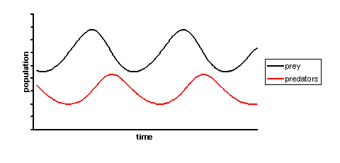
- The populations of predators and prey depend on each other.
- When there are many predators there are few prey. As the predators die off from lack of food, the prey population rebounds, enabling it to sustain a larger population of predators.
- This up and down cycle of populations can be well represented by differential equations and has a periodic solution.
Key Terms
- predator: any animal or other organism that hunts and kills other organisms (their prey), primarily for food
- prey: a living thing that is eaten by another living thing
- differential equation: an equation involving the derivatives of a function
The predator–prey equations are a pair of first-order, non-linear, differential equations frequently used to describe the dynamics of biological systems in which two species interact, one a predator and one its prey.
They evolve in time according to the pair of equations:
dtdx=αx−βxy
dtdy=δxy−γy
where
x is the number of prey (for example, rabbits);
y is the number of some predator (for example, foxes); and
dtdx and
dtdy represent the growth rates of the two populations over time;
t represents time; and
α,
β,
γ, and
δ are parameters describing the interaction of the two species.
The model makes a number of assumptions about the environment and evolution of the predator and prey populations:
- The prey population finds ample food at all times.
- The food supply of the predator population depends entirely on the prey populations.
- The rate of change of population is proportional to its size.
- During the process, the environment does not change in favor of one species and the genetic adaptation is sufficiently slow.
- As differential equations are used, the solution is deterministic and continuous. This, in turn, implies that the generations of both the predator and prey are continually overlapping.
The prey are assumed to have an unlimited food supply, and to reproduce exponentially unless subject to predation; this exponential growth is represented in the equation above by the term
αx. The rate of predation upon the prey is assumed to be proportional to the rate at which the predators and the prey meet; this is represented above by
βxy. If either
x or
y is zero, then there can be no predation. With these two terms, the equation above can be interpreted as follows: the change in the prey's number is given by its own growth minus the rate at which it is preyed upon.
In the predator equation,
δxy represents the growth of the predator population. (Note the similarity to the predation rate; however, a different constant is used as the rate at which the predator population grows is not necessarily equal to the rate at which it consumes the prey).
γy represents the loss rate of the predators due to either natural death or emigration; it leads to an exponential decay in the absence of prey. Hence, the equation expresses the change in the predator population as growth fueled by the food supply, minus natural death.
The equations have periodic solutions and do not have a simple expression in terms of the usual trigonometric functions. They can only be solved numerically. However, a linearization of the equations yields a solution similar to simple harmonic motion with the population of predators following that of prey by 90 degrees.
Licenses & Attributions
CC licensed content, Shared previously
CC licensed content, Specific attribution