Characteristics of Linear Functions
Learning Outcomes
- Identify important features of graphs of linear functions
[latex]\begin{array}{cc}\text{Equation form}\hfill & y=mx+b\hfill \\ \text{Function notation}\hfill & f\left(x\right)=mx+b\hfill \end{array}[/latex]
We previously learned how to calculate the slope given input and output values. Given two values for the input, [latex]{x}_{1}[/latex] and [latex]{x}_{2}[/latex], and two corresponding values for the output, [latex]{y}_{1}[/latex] and [latex]{y}_{2}[/latex] —which can be represented by a set of points, [latex]\left({x}_{1}\text{, }{y}_{1}\right)[/latex] and [latex]\left({x}_{2}\text{, }{y}_{2}\right)[/latex]—we can calculate the slope [latex]m[/latex], as follows[latex]m=\dfrac{\text{change in output (rise)}}{\text{change in input (run)}}=\dfrac{\Delta y}{\Delta x}=\dfrac{{y}_{2}-{y}_{1}}{{x}_{2}-{x}_{1}}[/latex]
where [latex]\Delta y[/latex] is the vertical displacement and [latex]\Delta x[/latex] is the horizontal displacement. In function notation, the corresponding values for the outputs [latex]{y}_{1}[/latex] and [latex]{y}_{2}[/latex] for the function [latex]f[/latex] are [latex]{y}_{1}=f\left({x}_{1}\right)[/latex] and [latex]{y}_{2}=f\left({x}_{2}\right)[/latex], so when using function notation we equivalently write[latex]m=\dfrac{f\left({x}_{2}\right)-f\left({x}_{1}\right)}{{x}_{2}-{x}_{1}}[/latex]
The slope of a function is calculated by the change in [latex]y[/latex] divided by the change in [latex]x[/latex]. It does not matter which coordinate is used as the [latex]\left({x}_{2,\text{ }}f({x}_{2}\right)[/latex] and which is the [latex]\left({x}_{1},\text{ }f({x}_{1}\right))[/latex], as long as each calculation is started with the elements from the same coordinate pair.[latex]m=\dfrac{f\left({x}_{2}\right)-f\left({x}_{1}\right)}{{x}_{2}-{x}_{1}}=\dfrac{f\left({x}_{1}\right)-f\left({x}_{2}\right)}{{x}_{1}-{x}_{2}}[/latex]
Calculating Slope
The slope, or rate of change, of a function [latex]m[/latex] can be calculated using the following formula: [latex-display]m=\dfrac{\text{change in output (rise)}}{\text{change in input (run)}}=\dfrac{\Delta y}{\Delta x}=\dfrac{{y}_{2}-{y}_{1}}{{x}_{2}-{x}_{1}}=\dfrac{f(x_{2})-f(x_{1})}{{x}_{2}-{x}_{1}}[/latex-display] where [latex]{x}_{1}[/latex] and [latex]{x}_{2}[/latex] are input values, [latex]{y}_{1}[/latex] and [latex]{y}_{2}[/latex] are output values.Example
If [latex]f\left(x\right)[/latex] is a linear function and [latex]f(3)=-2[/latex] and [latex]f(8)=1[/latex], find the slope. Is this function increasing or decreasing?Answer: We have been given two input and output values for [latex]f(x)[/latex]. [latex]f(3)=-2[/latex] corresponds to the coordinate pair [latex]\left(3,-2\right)[/latex] and [latex]f(8)=1[/latex] corresponds to the coordinate pair [latex]\left(8,1\right)[/latex]. To find the rate of change, we divide the change in output by the change in input.
[latex]m=\dfrac{\text{change in output}}{\text{change in input}}=\dfrac{f\left(8\right)-f\left(3\right)}{8-3}=\dfrac{1-\left(-2\right)}{8 - 3}=\dfrac{3}{5}[/latex]
We could also write the slope as [latex]m=0.6[/latex]. The function is increasing because [latex]m>0[/latex]. As noted earlier, the order in which we write the points does not matter when we compute the slope of the line as long as the first output value, or y-coordinate, used corresponds with the first input value, or x-coordinate, used.Vertical and Horizontal Lines
Vertical and horizontal lines are two special cases of linear equations. Recall that the equation of a vertical line is given as[latex]x=c[/latex]
where c is a constant. Regardless of the y-value of any point on the line, the x-coordinate of the point will be c. Consider a line containing the following points: [latex]\left(-3,-5\right),\left(-3,1\right),\left(-3,3\right)[/latex], and [latex]\left(-3,5\right)[/latex]. First, we will try to find the slope.[latex]m=\dfrac{5 - 3}{-3-\left(-3\right)}=\dfrac{2}{0}[/latex]
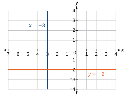
Zero in the denominator means that the slope is undefined. As a result, it is impossible to write the vertical line as an equation in the form [latex]y=mx+b[/latex]. Also, recall that a function must have exactly one output for every input. As a result, a vertical line is NOT a function. These points do not define a function because for our input, [latex]x=-3[/latex], we have an infinite number of outputs! Although these points cannot be defined as a function, we can nevertheless plot the points. You can see the line in the graph below. Notice that all of the x-coordinates are the same and we find a vertical line through [latex]x=-3[/latex]. The equation of a horizontal line is given as[latex]y=c[/latex]
where c is a constant. The slope of a horizontal line is zero, and for any x-value of a point on the line, the corresponding y-coordinate will be c. Suppose we want to find the equation of a line that contains the following set of points: [latex]\left(-2,-2\right),\left(0,-2\right),\left(3,-2\right)[/latex], and [latex]\left(5,-2\right)[/latex]. We can use point-slope form. First, we find the slope using any two points on the line.[latex]\begin{array}{l}m & =\dfrac{-2-\left(-2\right)}{0-\left(-2\right)}\hfill \\ & =\dfrac{0}{2}\hfill \\ & =0\hfill \end{array}[/latex]
The graph is a horizontal line through [latex]y=-2[/latex]. Notice that all of the y-coordinates are the same. The line [latex]x=−3[/latex] is a vertical line. The line [latex]y=−2[/latex] is a horizontal line.
Example
Find the equation of the line passing through the given points: [latex]\left(1,-3\right)[/latex] and [latex]\left(1,4\right)[/latex].Answer: The x-coordinate of both points is [latex]1[/latex]. Therefore, we have a vertical line, [latex]x=1[/latex]. This line cannot be defined as a function.
Contribute!
Licenses & Attributions
CC licensed content, Original
- Precalculus. Provided by: OpenStax Authored by: Jay Abramson, et al.. Located at: https://openstax.org/books/precalculus/pages/1-introduction-to-functions. License: CC BY: Attribution. License terms: Download For Free at : http://cnx.org/contents/[email protected]..
- Revision and Adaptation. Provided by: Lumen Learning License: CC BY: Attribution.
- Write and Graph a Linear Function by Making a Table of Values (Intro). Authored by: James Sousa (Mathispower4u.com) for Lumen Learning. License: CC BY: Attribution.
CC licensed content, Shared previously
- Ex: Find the Slope Given Two Points and Describe the Line. Authored by: James Sousa (Mathispower4u.com) . License: CC BY: Attribution.
- Ex: Slope Application Involving Production Costs. Authored by: James Sousa (Mathispower4u.com) . License: CC BY: Attribution.
